Bias Variance

Imports¶

Part 1: Approximation vs Learning¶

Cell 1.1: Approximation¶

Goal:

• Compare how well a constant model and a linear model can approximate the true target function $f(x) = \sin(\pi x)$ on $x \in [-1, 1]$, with no notion of training data yet

Implementation: cell1_approximation()

• Fits $g_0(x) = b$ and $g_1(x) = ax + b$ directly to the dense true function by least squares, in fit_constant_model()/fit_linear_model()
• Plots True function vs constant model and True function vs linear model, each shading the approximation error, plus a Comments panel with both models’ equations and errors

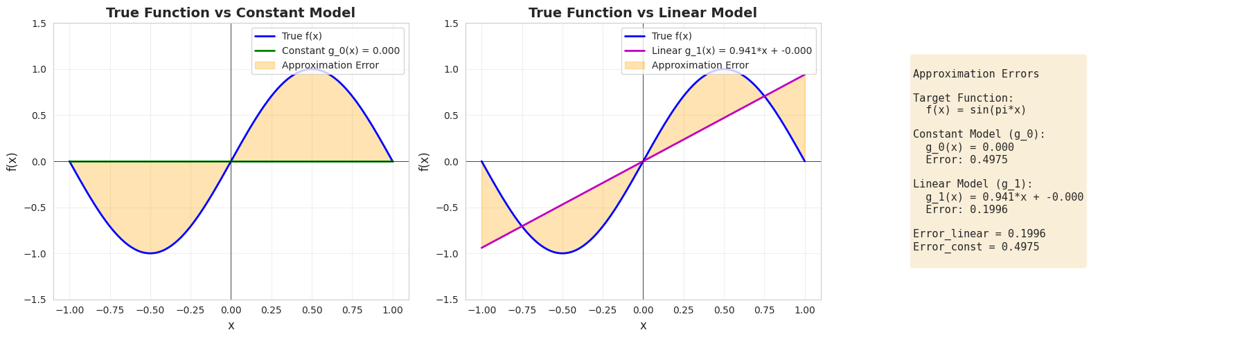
Cell 1.2: Learning once¶

Goal:

• Contrast learning from a small training set with the pure approximation of Cell 1.1, and separate in-sample error $E_{in}$ from out-of-sample error $E_{out}$

Implementation: cell2_learning_once()

• Draws N_samples random training points and fits $g_0$/$g_1$ to them with fit_models_and_predict()
• Computes $E_{in}$ (error on the training points) and $E_{out}$ (error against the true function) for both models

Usage

• Inputs

  • seed: random seed for the training points sampled
  • N_samples: number of training points, 2-20

• Panels

  • Constant model: $f(x)$, the fitted $g_0$, and the training points, titled with $E_{in}$/$E_{out}$
  • Linear model: $f(x)$, the fitted $g_1$, and the training points, titled with $E_{in}$/$E_{out}$
  • Comments: current seed, N_samples, and both models’ $E_{in}$/$E_{out}$

Guided usage

• Leave N_samples at 2 and change seed a few times
  • Observe the linear model reaches $E_{in} = 0$ on almost every draw (2 points fully determine a line), yet $E_{out}$ still varies widely
• Raise N_samples from 2 toward 20
  • Observe $E_{in}$ for the linear model rise off zero, while $E_{out}$ for both models settles down: fitting 2 points perfectly is not the same as learning $f$

Part 2: Bias-Variance Decomposition¶

Cell 2.1: Learning: bias-variance decomposition¶

Goal:

• Repeat Cell 1.2’s experiment across many random training sets, and read bias and variance off how the resulting models scatter around $f$

Implementation: cell3_learning_bias_variance()

• Runs N_experiments independent draws of N_samples points, refitting $g_0$ and $g_1$ each time
• Overlays every fitted model in translucent lines, plus the average model as a dashed line, so bias (average vs $f$) and variance (spread around the average) are both visible at once

Usage

• Inputs

  • seed: random seed for the experiments
  • N_samples: training points per experiment, 2-20
  • N_experiments: number of repeated experiments, 5-100

• Panels

  • Constant models: $f(x)$, every fitted $g_0$, and their average
  • Linear models: $f(x)$, every fitted $g_1$, and their average
  • Comments: average $E_{in}$/$E_{out}$ and the bias-variance reading for both models

Guided usage

• Compare the two panels at the default N_samples = 2
  • Observe the constant lines cluster tightly (low variance) but sit far from $f$ (high bias), while the linear lines spread widely (higher variance) but average closer to $f$ (lower bias)
• Raise N_experiments toward 100
  • Observe the average line in each panel stabilize, giving a more reliable bias estimate without changing how spread out the individual fits are

Cell 2.2: Learning plots: bias-variance vs training set size¶

Goal:

• Trace how $E_{in}$, $E_{out}$, $\text{bias}^2$, and variance move as training set size grows, for both models at once

Implementation: cell4_learning_plots()

• Repeats Cell 2.1’s experiment at every training size from 2 up to max_N_samples, averaging N_experiments trials at each size
• Plots the four error curves for $g_0$ and $g_1$ side by side, verifying $E_{out} \approx \text{Bias}^2 + \text{Variance}$ for this noise-free target

Usage

• Inputs

  • seed: random seed, fixed across training sizes for a fair comparison
  • N_experiments: experiments averaged per training size, 20-200
  • max_N_samples: largest training size swept, 5-30

• Panels

  • Constant model (g_0), bias-variance analysis: $E_{in}$, $E_{out}$, $\text{Bias}^2$, and variance vs training size
  • Linear model (g_1), bias-variance analysis: the same four curves for $g_1$
  • Comments: the decomposition formula and both models’ values at max_N_samples

Guided usage

• Raise max_N_samples toward 30
  • Observe variance keep shrinking toward 0 for both models, while each model’s bias curve flattens out at its own level
• Compare the flattened bias level between panels
  • Observe the linear model’s bias floor sits below the constant model’s: more model capacity lowers bias, at the cost of the variance seen in Cell 2.1

Part 3: Bias-Variance With Noise¶

Cell 3.1: Learning with noise: bias-variance decomposition¶

Goal:

• Repeat Cell 2.1’s multi-experiment view with Gaussian noise added to the training labels, $y = f(x) + \mathcal{N}(0, \sigma^2)$

Implementation: cell5_learning_with_noise()

• Adds noise of standard deviation noise_std to each training draw before fitting $g_0$/$g_1$, otherwise identical to cell3_learning_bias_variance()

Usage

• Inputs

  • seed: random seed for the experiments
  • noise_std: standard deviation $\sigma$ of the label noise, 0-0.5
  • N_samples: training points per experiment, 2-20
  • N_experiments: number of repeated experiments, 5-100

• Panels

  • Constant models: $f(x)$, every fitted $g_0$, and their average
  • Linear models: $f(x)$, every fitted $g_1$, and their average
  • Comments: average $E_{in}$/$E_{out}$ for both models at the current noise level

Guided usage

• Leave noise_std at 0 and compare against Cell 2.1
  • Observe the two panels match Cell 2.1 exactly: zero noise recovers the noise-free case
• Raise noise_std from 0 toward 0.5
  • Observe both panels spread out further and $E_{out}$ climb for both models, since every fit now chases noise the true function never had

Cell 3.2: Learning plots with noise: bias-variance vs training set size¶

Goal:

• Trace $E_{in}$, $E_{out}$, $\text{bias}^2$, and variance against training set size, as in Cell 2.2, now with noisy training labels

Implementation: cell6_learning_plots_with_noise()

• Repeats Cell 2.2’s sweep with noise_std added to every training draw before fitting, over N_samples from 2 up to the current slider value

Usage

• Inputs

  • seed: random seed, fixed across training sizes
  • noise_std: standard deviation $\sigma$ of the label noise, 0-0.5
  • log(N_samples) (log scale): largest training size swept, 2-256
  • log(N_experiments) (log scale): experiments averaged per training size, 16-1024

• Panels

  • Constant model (g_0), bias-variance analysis: $E_{in}$, $E_{out}$, $\text{Bias}^2$, and variance vs training size
  • Linear model (g_1), bias-variance analysis: the same four curves for $g_1$
  • Comments: the noisy decomposition formula and both models’ values at the largest training size

Guided usage

• Set noise_std to 0.1 or 0.2 and compare against Cell 2.2
  • Observe both $E_{out}$ curves shift up by roughly $\sigma^2$, while the bias curves barely move: noise adds an irreducible floor, it does not change what the model class can represent
• Raise log(N_samples) toward its maximum with noise still on
  • Observe variance keeps shrinking as before, but $E_{out}$ levels off above 0: more data cannot remove the noise term, only the variance term