- This notebook teaches how to compute exact posteriors in a discrete Bayesian network
- Concepts are built on the the burglary-alarm network and the query
- The flow is:
- Inference by enumeration (brute force)
- Variable elimination (caching)
- Irrelevant-variable pruning
- Complexity and limits
Imports
%load_ext autoreload
%autoreload 2

# System libraries.
import logging

# Third-party libraries.
The autoreload extension is already loaded. To reload it, use:
%reload_ext autoreload
# Use this for most notebooks.
import helpers.hintrospection as hintros
import helpers.htutorial as htutori

import L06_01_exact_inference_utils as utils

htutori.config_notebook()

# Initialize logger.
_LOG = logging.getLogger(__name__)
utils.init_loggers(_LOG)

# Convert `display` into `print()` when running outside IPython.
try:
    from IPython.display import display
except ImportError:
    display = print  # type: ignore
/opt/venv/lib/python3.12/site-packages/pgmpy/estimators/__init__.py:4: FutureWarning: `pgmpy.estimators.StructureScore` is deprecated and will be removed in v1.3.0. Use `pgmpy.structure_score` instead.
from .StructureScore import (
pymc is not installed
arviz is not installed
preliz is not installed
sns is not installed
Python 3.12.13
Linux 7f4d4ef8cf8c 6.12.67-linuxkit #1 SMP Sun Jan 25 02:26:28 UTC 2026 aarch64 GNU/Linux
---------------------------------------------------------------------------
NameError                                 Traceback (most recent call last)
Cell In[1], line 9
      5
      6 htutori.config_notebook()
      7
      8 # Initialize logger.
----> 9 _LOG = logging.getLogger(__name__)
     10 utils.init_loggers(_LOG)
     11
     12 # Convert `display` into `print()` when running outside IPython.

NameError: name 'logging' is not defined
Part 1: Setting Up the Inference Problem
Cell 1.1: The burglary alarm network and its CPTs
Goal:
- Ground every later inference step in one concrete network: the burglary-alarm story and its five conditional probability tables
- The five variables are:
- Root causes: , (blue)
- The (orange)
- The calls: , (purple)
- The joint factorizes into five small CPTs:
Implementation: cell1_1_show_network_and_cpts()
- Draws the DAG colored by role, prints the priors /, the table, and the two call CPTs
# Display the DAG and its five conditional probability tables.
utils.cell1_1_show_network_and_cpts()

# TODO(ai_gp): The prob for P(Alarm | Burglary, Earthquake) do not match
# the slides in L06.1
# TODO(ai_gp): The colors of the nodes are different than the slides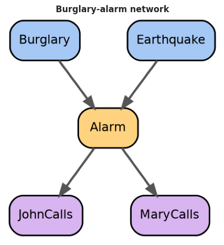
Priors on the root causes:
P(Alarm | Burglary, Earthquake):
P(JohnCalls | Alarm) and P(MaryCalls | Alarm):
- The joint over five variables factorizes into five small CPTs
- Calls depend on the world only through : they are conditionally independent of and given
- Storing 5 small CPTs (10 independent numbers) is far cheaper than the full joint ( numbers)
- Inference never touches the full joint directly: it works with the factored form, a product of the small CPTs attached to each node
Cell 1.2: Query, evidence, and hidden variables
Goal:
- Build intuition for which variables must be summed out, by letting students pick the query and mark any subset of nodes as evidence
Implementation: cell1_2_query_roles_widget()
- Recolors the DAG by role, query/evidence/hidden, for the current
choice of
Query Xand observed nodes, via_read_query() - Restates the query in math and counts the hidden terms in the Comments panel
hintros.print_obj_info(utils.cell1_2_query_roles_widget)Usage
Inputs
Query X: which node is being asked aboutobserve <node>: one checkbox plus True/False value per node, marking it as evidence
Panels
Roles for the current query: the DAG recolored by role: query (blue), evidence (red), hidden (grey)Comments: the query restated in math, and the hidden-term count
# Assign each node a role and recolor the DAG for the current query.
utils.cell1_2_query_roles_widget()Guided usage
- Mark every node except
Query Xas evidence- Observe no node stays hidden, and the term count in Comments drops to : nothing needs to be summed out
- Uncheck every evidence box, leaving only
Query Xset- Observe every other node turns hidden, and the term count climbs to 24: the posterior we want, , still has to marginalize all of them away, they cannot simply be dropped
Part 2: Inference by Enumeration
Cell 2.1: From conditional to joint via normalization
Goal:
- Derive why a conditional query reduces to summing the joint and rescaling by a normalization constant
Implementation: cell2_1_normalization_widget()
- Fixes the canonical query and
computes both the unnormalized joint and the normalized posterior with
_enumerate_posterior() show normalizationswitches the middle panel between the two views
hintros.print_obj_info(utils.cell2_1_normalization_widget)Usage
Inputs
show normalization: toggle between the unnormalized joint and the normalized posterior
Panels
Derivation: the three equation lines from down to the alarm-network sumUnnormalized joint/Normalized posterior: bars for =T/F in whichever view is toggled onComments: the unnormalized values, , and the resulting posterior
# Toggle between the unnormalized joint and the normalized posterior.
utils.cell2_1_normalization_widget()Guided usage
- Toggle
show normalizationoff, then on- Observe the bars change scale (they no longer sum to 1) but keep the same relative height: rescaling by never changes which value is more likely, only the units
- Read off the Comments panel
- Observe : exactly the constant that makes the posterior sum to 1, computed without ever touching directly
Cell 2.2: Computing the posterior by enumeration
Goal:
- Compute the exact posterior by hand, summing CPT products over the
hidden variables, and confirm it against the
pgmpyengine
Implementation: cell2_2_enumeration_widget()
- Enumerates every hidden assignment and its CPT product with
_enumerate_posterior(), for the currentQuery X/evidence - Cross-checks the result against
pgmpy’sVariableEliminationreference
hintros.print_obj_info(utils.cell2_2_enumeration_widget)Usage
Inputs
Query X: which node is being asked aboutobserve <node>: one checkbox plus True/False value per node, marking it as evidence
Panels
Sum for X=T/Sum for X=F: every hidden assignment and its CPT product, for each query valuePosterior: the resulting bars, with thepgmpyreference overlaid in dashed redComments: hidden-variable count, row count summed, and whether the two engines agree
# Compute the posterior by enumeration and validate against pgmpy.
utils.cell2_2_enumeration_widget()Guided usage
- Mark one more node as evidence, then another
- Observe the row count in Comments halve each time: one fewer hidden variable means one fewer factor of 2 in
- Compare the enumeration bars against the dashed
pgmpyreference for several different queries- Observe they always coincide: hand enumeration and the library engine compute the same posterior, e.g. the famous result
Cell 2.3: Visualizing the enumeration tree
Goal:
- Expose the enumeration computation as a tree, to see the repeated subexpressions that motivate variable elimination
Implementation: cell2_3_enumeration_tree_widget()
- Draws the two-level branch tree over the hidden
Earthquake/Alarmvalues, for the fixed query - Colors each leaf’s shared factor by the value
of
Alarmon that branch, when highlighting is on
hintros.print_obj_info(utils.cell2_3_enumeration_tree_widget)Usage
Inputs
Sum order: which hidden variable branches first,EarthquakeorAlarmhighlight repeated work: color leaves by their shared factor
Panels
Enumeration evaluation tree: the branch tree, leaves labeled by their CPT productComments: the operation count and why the repeats are wasteful
# Draw the enumeration tree and highlight the repeated subexpressions.
utils.cell2_3_enumeration_tree_widget()Guided usage
- Turn on
highlight repeated work- Observe leaves under different first-level branches share the same
color whenever
Alarmagrees: the identical factor is recomputed in more than one branch
- Observe leaves under different first-level branches share the same
color whenever
- Switch
Sum orderbetween the two options- Observe the tree’s shape changes, but the same repeated-factor pattern persists either way: caching it once, instead of recomputing it per branch, is the one idea behind variable elimination
Part 3: Variable Elimination
Cell 3.1: Factors as the unit of computation
Goal:
- Introduce the factor, a table over a subset of variables, as the single data structure variable elimination manipulates
Implementation: cell3_1_factor_operations_widget()
- Renders the chosen CPT as a
Factortable, then marginalizes outSum outwithpgmpy’sfactor.marginalize()
hintros.print_obj_info(utils.cell3_1_factor_operations_widget)Usage
Inputs
Factor: which CPT to view as a factor, labeled by its scopeSum out: which variable in that factor’s scope to marginalize away
Panels
Before: the selected factor’s table and scopeAfter summing out <var>: the same factor once that variable is marginalized outComments: how many rows the table shrank by, and the two operations inference needs
# Explore factors and the summing-out operation.
utils.cell3_1_factor_operations_widget()
Guided usage
- Pick a factor with a scope of 3 variables, then sum out one of them
- Observe the row count drop from 8 to 4: summing out one variable halves the table, one dimension at a time
- Switch
Factorto a CPT with only 1 variable in scope- Observe
Sum outleaves a(scalar)factor: summing out every remaining variable collapses the table to a single number
- Observe
Cell 3.2: Variable elimination step by step
Goal:
- Walk through variable elimination on the alarm query, one elimination at a time, and compare its operation count against enumeration
Implementation: cell3_2_variable_elimination_widget()
- Advances
stepthrough_variable_elimination_steps(), which eliminates hidden variables in the chosenOrderand caches each new factor - Tallies multiplications and additions used so far, against the fixed enumeration operation count
hintros.print_obj_info(utils.cell3_2_variable_elimination_widget)Usage
Inputs
Order: which hidden variable,EarthquakeorAlarm, is eliminated firstelimination step: how many variables have been eliminated so far, 0-2
Panels
Active factors (step N): the current factor scopesNew factor: the factor created at this step, or “no elimination yet” at step 0Posterior and op count: the running posterior next to the enumeration-vs-VE operation comparisonComments: order, step, and both operation counts
# Step through variable elimination one variable at a time.
utils.cell3_2_variable_elimination_widget()
Guided usage
- Advance
elimination stepfrom 0 to 2- Observe the active-factor list shrink by one each step, while the posterior bars never change: the final answer is fixed from the start, only the work to reach it is staged
- Compare the VE operation total in Comments against the enumeration
count
- Observe VE finishes with noticeably fewer operations, by reusing each cached factor instead of recomputing it per branch
Cell 3.3: Pruning irrelevant variables
Goal:
- Show that a variable which is not an ancestor of the query or evidence can be deleted before any computation, for free
Implementation: cell3_3_pruning_widget()
- Builds an extended network with an extra
Neighborleaf, then shades nodes by whether they are the query, evidence, or an ancestor of either prune irrelevant variablescompares the posterior on the full network against the posterior on the ancestor-only subgraph
hintros.print_obj_info(utils.cell3_3_pruning_widget)Usage
Inputs
Query X: which node is being asked about, over the extended networkobserve <node>: one checkbox plus True/False value per nodeprune irrelevant variables: toggle between the full and pruned network
Panels
Relevant (green) vs irrelevant (grey): the DAG shaded by relevance to the current query/evidenceFull vs pruned posterior: bars for both networks, side by sideComments: the irrelevant nodes and whether the two posteriors match
# Shade nodes by relevance and compare full vs pruned posteriors.
utils.cell3_3_pruning_widget()
Guided usage
- Leave
Neighborunobserved and toggleprune irrelevant variableson and off- Observe the posterior bars stay identical either way, while
Comments lists
Neighboras irrelevant: an unobserved effect node with no bearing on the query contributes nothing
- Observe the posterior bars stay identical either way, while
Comments lists
- Mark
Neighboras evidence- Observe it turns green (relevant) and pruning stops removing it: an observed node is never irrelevant, however far it sits from the query
Part 4: Complexity and Limits
Cell 4.1: Complexity: polytrees vs general graphs
Goal:
- Make concrete that exact inference is cheap on tree-shaped networks and blows up on densely connected ones
Implementation: cell4_1_complexity_widget()
- Draws a chain (
polytree) and a fully connected graph of the samen, then plots vs operation-count curves withOrder qualityscaling the constant
hintros.print_obj_info(utils.cell4_1_complexity_widget)Usage
Inputs
n: number of nodes in both example graphs, 3-10Structure: which curve the marked operating point sits on,polytreeorfully connectedOrder quality:goodorbad, scaling the cost constant
Panels
Polytree (n=N): a chain network of the chosen sizeDense network (n=N): a fully connected network of the same sizeCost vs network size: the two cost curves on a log y-axis, with the current operating point markedComments: the operating-point cost and the role of order quality
# Compare exact-inference cost on polytrees vs dense networks.
utils.cell4_1_complexity_widget()Guided usage
- Raise
nfrom 3 toward 10 withStructureset tofully connected- Observe the marked point climb the exponential curve, while the
same raise under
polytreebarely moves the point on the linear curve
- Observe the marked point climb the exponential curve, while the
same raise under
- Switch
Order qualityfromgoodtobad- Observe the operating-point cost jump higher at the same
n: a worse elimination order inflates the constant in front of both curves
- Observe the operating-point cost jump higher at the same
Cell 4.2: When exact inference breaks down
Goal:
- Summarize the three regimes where exact inference is the right tool, or is not, and motivate the approximate methods covered next
Implementation: cell4_2_breakdown_widget()
- Looks up the chosen
Scenarioin a fixed regime table and highlights its row and recommendation
hintros.print_obj_info(utils.cell4_2_breakdown_widget)Usage
Inputs
Scenario:Small discrete polytree,Large dense discrete network, orContinuous variables
Panels
Regimes for exact inference: the three-regime comparison table, with the current scenario’s row highlightedContinuous case: a small DAG sketch showingComments: the recommendation banner,EXACTorAPPROXIMATE, and why
# Select a regime and read off the exact-vs-approximate recommendation.
utils.cell4_2_breakdown_widget()Guided usage
- Step through all three
Scenariooptions- Observe only
Small discrete polytreerecommendsEXACT; both other scenarios recommendAPPROXIMATE, for two different reasons: an exponential cost blowup, or a sum that is not even a finite sum
- Observe only
- Compare this recommendation table against Cell 4.1’s cost curves
- Observe the
Large dense discrete networkrow is exactly the regime where Cell 4.1’s exponential curve makes exact inference impractical
- Observe the