SHAP API

A guided exploration of SHAP (SHapley Additive exPlanations):

Explainer: wraps a trained ML model and computes Shapley values
Explanation: holds SHAP values, baseline prediction, and feature data
Plots: visualize feature contributions locally (per prediction) and globally

Imports and Setup¶

%load_ext autoreload
%autoreload 2

import logging
import warnings

import matplotlib.pyplot as plt
import numpy as np
import pandas as pd
import shap

import sklearn.datasets
import sklearn.linear_model

warnings.filterwarnings("ignore")

import helpers.hdbg as hdbg
import helpers.hnotebook as hnotebo

hdbg.init_logger(verbosity=logging.INFO)
_LOG = logging.getLogger(__name__)
hnotebo.config_notebook()

try:
    from IPython.display import display
except ImportError:
    display = print  # type: ignore

WARNING: Running in Jupyter
INFO  > cmd='/opt/venv/lib/python3.12/site-packages/ipykernel_launcher.py -f /root/.local/share/jupyter/runtime/kernel-e30c7a25-5152-4b1f-96fc-83f236f291da.json'

Library Overview¶

What problem it solves:
- Modern ML models (tree ensembles, neural nets) are accurate but opaque
- SHAP answers “why did the model predict X?” for any single prediction
- Decomposes predictions into per-feature contributions grounded in game theory (Shapley values from cooperative game theory)
Key abstraction:
- Every prediction = baseline + sum of per-feature SHAP values
- Shapley values satisfy consistency, dummy, and efficiency axioms (no other attribution satisfying all three exists)

Mental model:

Object	Description	Shape / Type
`model`	Trained ML model	`X -> prediction`
`Explainer(model, background)`	Configured explainer	Wraps model + background data
`explainer(X)`	Explanation for batch	Returns Explanation object
`Explanation.values`	SHAP contributions per feature	`(n_samples, n_features)` array
`Explanation.base_values`	Model’s average output	`(n_samples,)` array, usually constant
`Explanation.data`	Original input features	`(n_samples, n_features)` array
`prediction[i]`	Additive decomposition	`base_values[i] + values[i].sum()`

Key classes:
- shap.LinearExplainer: exact for linear models (used throughout this notebook)
- shap.TreeExplainer: fast and exact for tree-based models
- shap.KernelExplainer: model-agnostic, works with any callable
- shap.Explanation: result object (values, base_values, data)

Part 1: Toy Data Setup¶

Cell 1.1: Create a toy regression dataset¶

Goal:

Build the minimal dataset needed to explore all SHAP primitives
Use regression (not classification) to keep SHAP values 2D and easy to inspect

# Four named features, 30 samples, pure regression target.
np.random.seed(42)
X, y = sklearn.datasets.make_regression(
    n_samples=30,
    n_features=4,
    n_informative=3,
    noise=10.0,
    random_state=42,
)
X_df = pd.DataFrame(X, columns=["age", "income", "debt", "employment"])
y_s = pd.Series(y, name="target")

print("X_df.shape=", X_df.shape)
print("y_s.shape=", y_s.shape)
display(X_df.head(3))

X_df.shape= (30, 4)
y_s.shape= (30,)

# Feature statistics: central tendency, spread, and range.
print("=== Feature Statistics ===")
print(X_df.describe())

# Correlations between features and target.
print("=== Correlations with target ===")
corr_with_target = X_df.corrwith(y_s).sort_values(ascending=False)
display(corr_with_target)

# Pairwise correlations between all features as a heatmap.
import seaborn as sns

print("=== Feature Correlations ===")
fig, ax = plt.subplots(figsize=(8, 6))
corr_matrix = X_df.corr()
sns.heatmap(
    corr_matrix,
    annot=True,
    fmt=".3f",
    cmap="coolwarm",
    center=0,
    ax=ax,
    square=True,
)
ax.set_title("Feature Correlation Matrix")
plt.tight_layout()
plt.show()
plt.close("all")

Cell 1.2: Train a linear regression model¶

Goal:

Train a LinearRegression model on the toy dataset
This is the single model we will explain end-to-end throughout the notebook

# Train linear regression model.
linear_model = sklearn.linear_model.LinearRegression()
linear_model.fit(X_df, y_s)
print("linear_model=", linear_model)

linear_model= LinearRegression()

# Show linear model coefficients and intercept.
coef_df = pd.DataFrame(
    {
        "feature": X_df.columns,
        "coefficient": linear_model.coef_,
    }
)
coef_df["abs_coef"] = np.abs(coef_df["coefficient"])
display(coef_df.sort_values("abs_coef", ascending=False))
print(f"Intercept: {linear_model.intercept_:.6f}")

Intercept: 3.158971

Part 2: Primitive 1 - The Explainer¶

Cell 2.1: Construct a LinearExplainer¶

Mental model:

LinearExplainer wraps a linear model together with background data
Background data captures feature means and covariances used to compute conditional expectations
For a linear model $f(x) = w \cdot x + b$ , the SHAP value for feature $j$ is exactly $w_j \cdot (x_j - E[x_j])$

# Background data: statistics used to compute baseline expectations.
#
# Background data defines the reference distribution for computing SHAP values.
# LinearExplainer uses background data to estimate the expected value (baseline)
# and feature covariances.
#
# Key insight: SHAP values measure deviations from the baseline (expected value).
# The background data determines what "normal" or "average" means in your dataset.
#
# For LinearExplainer:
# - expected_value = mean of model(X) over background data
# - SHAP[i, j] = model_coef[j] * (X[i, j] - mean(background[:, j]))
#
# Larger background sets give more stable estimates but slower computation.
# Smaller background sets (e.g., 100-1000 samples) are often sufficient.
print("Background data usage:")
print("  - Establishes baseline: E[model(X)] = expected_value")
print("  - Computes feature means for centering")
print("  - For tree models: encodes feature interaction structure")
print("  - For kernel explainers: enables conditional expectation estimation")

# Construct LinearExplainer with model and background data.
linear_explainer = shap.LinearExplainer(linear_model, X_df)
print("type(linear_explainer)=", type(linear_explainer))
print("linear_explainer.expected_value=", linear_explainer.expected_value)

type(linear_explainer)= <class 'shap.explainers._linear.LinearExplainer'>
linear_explainer.expected_value= -12.996543788805079

Cell 2.2: Inspect the LinearExplainer¶

# expected_value is E[model(X)], the global baseline.
print("linear_explainer.expected_value=", linear_explainer.expected_value)
print("mean of y (approx baseline)=", round(y_s.mean(), 4))
# Interpretation: expected_value equals the model's average prediction over the
# training set, which is the intercept offset from the mean-centered features.
print("\nInterpretation: expected_value = model's average output (~mean of y).")
print("SHAP values = deviations from this baseline for each feature.")

linear_explainer.expected_value= -12.996543788805079
mean of y (approx baseline)= -12.9965

Interpretation: expected_value = model's average output (~mean of y).
SHAP values = deviations from this baseline for each feature.

# Public interface of the LinearExplainer.
# Display all public methods with their signatures and docstrings.
import helpers.hintrospection as hintros

hintros.print_obj_info(linear_explainer)

Part 3: Primitive 2 - The Explanation Object¶

Explanation object: The central data structure for SHAP An Explanation bundles three key arrays:

.values: SHAP contributions
- shape: n_samples x n_features
- How much each feature “pushed” the prediction away from baseline
- Positive = increases prediction, Negative = decreases prediction
.base_values: Model’s average output
- shape: n_samples, all usually identical
- The expected value / baseline prediction
- Same for all samples unless model has per-sample defaults
.data: Original input features
- shape: n_samples x n_features
- Needed for plots that correlate feature value with SHAP impact

Additive property:

prediction[i] = base_values[i] + sum(values[i, :])

This always holds exactly for tree and linear explainers.

Cell 3.1: Compute SHAP values (get an `Explanation`)¶

Mental model:

Calling explainer(X) returns an Explanation object
This bundles SHAP values, baseline, and original data into one structure
For LinearExplainer, SHAP values are exact (no sampling)

# Compute SHAP values for all 30 samples using LinearExplainer.
explanation = linear_explainer(X_df)
print("type(explanation)=", type(explanation))

type(explanation)= <class 'shap._explanation.Explanation'>

Cell 3.2: Inspect `Explanation.values`¶

# .values: SHAP contribution of each feature for each sample.
print("type(explanation.values)=", type(explanation.values))
print("explanation.values.shape=", explanation.values.shape)
# Rows = samples, columns = features.
values_df = pd.DataFrame(explanation.values, columns=X_df.columns)
display(values_df.head(3))

type(explanation.values)= <class 'numpy.ndarray'>
explanation.values.shape= (30, 4)

Cell 3.3: Inspect `Explanation.base_values`¶

# .base_values: model's expected output (same for all samples).
print("explanation.base_values.shape=", explanation.base_values.shape)
print("explanation.base_values[0]=", round(explanation.base_values[0], 4))
print(
    "all identical?",
    np.allclose(explanation.base_values, explanation.base_values[0]),
)

explanation.base_values.shape= (30,)
explanation.base_values[0]= -12.9965
all identical? True

Cell 3.4: Inspect `Explanation.data`¶

# .data: the original feature values passed to the explainer.
print("type(explanation.data)=", type(explanation.data))
print("explanation.data.shape=", explanation.data.shape)
display(pd.DataFrame(explanation.data, columns=X_df.columns).head(3))

type(explanation.data)= <class 'numpy.ndarray'>
explanation.data.shape= (30, 4)

Cell 3.5: Verify the additive decomposition¶

Key invariant:

prediction[i] = base_value + sum(shap_values[i])
This always holds exactly for TreeExplainer (and LinearExplainer)

# Verify additive decomposition for sample index 0.
idx = 0
model_pred = linear_model.predict(X_df.iloc[[idx]])[0]
shap_sum = explanation.base_values[idx] + explanation.values[idx].sum()
print("model_pred=", round(model_pred, 6))
print("base + sum(shap)=", round(shap_sum, 6))
print("match?", np.isclose(model_pred, shap_sum))

model_pred= -44.844696
base + sum(shap)= -44.844696
match? True

Part 4: Primitive 3 - SHAP Plots¶

Cell 4.1: Waterfall plot (single prediction)¶

Goal:

See how each feature pushes prediction above or below the baseline for one sample
Start at E[f(X)] (bottom), end at f(x) (model output)

# Waterfall plot for sample 0: shows individual feature contributions.
shap.plots.waterfall(explanation[0])
plt.close("all")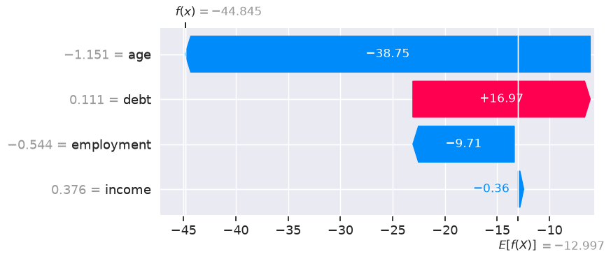

Key observations:

Each horizontal bar = one feature’s SHAP contribution
Red: feature pushes prediction up
Blue: feature pushes prediction down
Total = base_value + signed sum of all bars = model output

Cell 4.2: Bar plot (global feature importance)¶

Goal:

Rank features by their average absolute SHAP value across all samples
This is the global view: which features matter most overall?

# Bar plot: mean |SHAP value| per feature across all samples.
shap.plots.bar(explanation)
plt.close("all")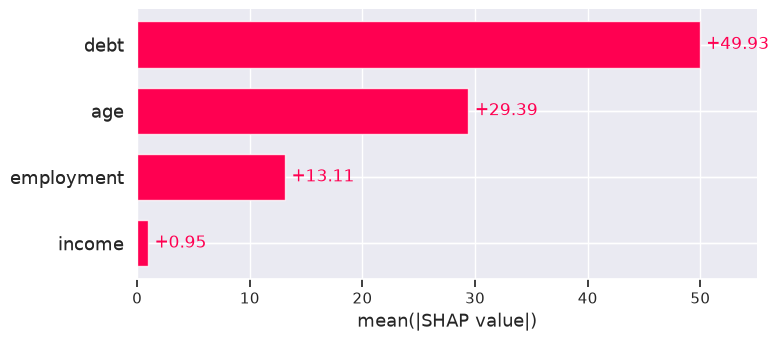

Key observations:

Bar length = mean(|SHAP value|) averaged across 30 samples
Longer bar = feature matters more globally
Does not show direction (sign), only magnitude

Cell 4.3: Beeswarm plot (global distribution of SHAP values)¶

Goal:

Show the distribution of SHAP values per feature across all samples
Color encodes the feature value (red = high, blue = low)

# Beeswarm: one dot per (sample, feature), color = feature value.
shap.plots.beeswarm(explanation)
plt.close("all")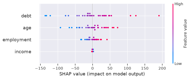

Key observations:

Each dot = one sample’s SHAP value for a given feature
Horizontal spread = range of SHAP contributions for that feature
Red dots with high SHAP -> high feature value increases the prediction
Blue dots with low SHAP -> low feature value decreases the prediction

Cell 4.4: Scatter plot (feature dependence)¶

Goal:

See how a single feature’s value relates to its SHAP contribution
Reveals linear, monotonic, or threshold-based effects

# Scatter: x = feature value, y = SHAP contribution for "income".
shap.plots.scatter(explanation[:, "income"])
plt.close("all")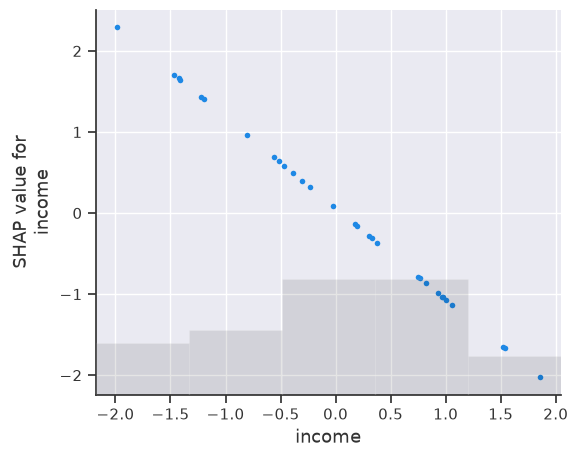

Key observations:

x-axis: raw feature value (income)
y-axis: SHAP contribution for income
A diagonal line -> monotonic effect; an S-curve -> threshold or saturation

Part 5: API Patterns¶

Cell 5.1: Local explanation for a specific sample¶

Build a per-sample breakdown table of feature values and their SHAP contributions.

# Table: feature value, SHAP value, and absolute SHAP for sample 5.
sample_idx = 5
local_df = pd.DataFrame(
    {
        "feature_value": X_df.iloc[sample_idx].values,
        "shap_value": explanation.values[sample_idx],
        "abs_shap": np.abs(explanation.values[sample_idx]),
    },
    index=X_df.columns,
).sort_values("abs_shap", ascending=False)
display(local_df)

Cell 5.2: Global importance as a sorted DataFrame¶

Rank features by mean absolute SHAP value across all samples.

# Global feature ranking by mean absolute SHAP.
global_importance_df = pd.DataFrame(
    {
        "feature": X_df.columns,
        "mean_abs_shap": np.abs(explanation.values).mean(axis=0),
        "mean_shap": explanation.values.mean(axis=0),
    }
).sort_values("mean_abs_shap", ascending=False)
display(global_importance_df)

Cell 5.3: Sign of SHAP values¶

Positive SHAP: feature increases prediction above baseline
Negative SHAP: feature decreases prediction below baseline

# Count positive vs negative SHAP values per feature across all samples.
sign_df = pd.DataFrame(
    {
        "n_positive": (explanation.values > 0).sum(axis=0),
        "n_negative": (explanation.values < 0).sum(axis=0),
    },
    index=X_df.columns,
)
display(sign_df)

Part 6: Other Explainer Types¶

This notebook used LinearExplainer end-to-end because it gives exact, interpretable SHAP values for linear models. SHAP also provides two other key explainer types:

shap.TreeExplainer: for tree-based models (decision trees, random forests, gradient boosting)
- Traverses the tree structure to compute exact Shapley values in polynomial time
- No background data required: the tree encodes the full conditional distribution
- Usage: expl = shap.TreeExplainer(tree_model)
shap.KernelExplainer: model-agnostic, works with any callable
- Approximates Shapley values by sampling perturbations of the input
- Slower than TreeExplainer but works with any model (sklearn, TensorFlow, etc.)
- Requires a small background dataset (often summarized with shap.kmeans)
- Usage: expl = shap.KernelExplainer(model.predict, shap.kmeans(X_df, k=5))

All three explainers share the same interface: call with data, get back an Explanation object with .values, .base_values, and .data. The additive decomposition prediction[i] = base_values[i] + values[i].sum() holds for all of them.

Part 7: Summary¶

Summary: The Mental Model¶

LinearExplainer (main focus): exact SHAP values for linear models; SHAP value for feature $j$ is $w_j \cdot (x_j - E[x_j])$ ; requires the trained model and background data
Explanation object: the central data structure with three arrays: .values (SHAP contributions, shape (n_samples, n_features)), .base_values (model’s average prediction), and .data (input feature values)
Additive decomposition: prediction[i] = base_values[i] + values[i].sum() holds exactly for LinearExplainer — SHAP values are a faithful partition of each prediction
Plots: waterfall for single-prediction breakdown, bar for global magnitude ranking, beeswarm for global distribution with direction, and scatter for feature-level dependence analysis
Other explainers: TreeExplainer for tree-based models (exact, fast), KernelExplainer for any callable (approximate, model-agnostic) — all share the same Explanation interface

Imports and Setup¶

Library Overview¶

Part 1: Toy Data Setup¶

Cell 1.1: Create a toy regression dataset¶

Cell 1.2: Train a linear regression model¶

Part 2: Primitive 1 - The Explainer¶

Cell 2.1: Construct a LinearExplainer¶

Cell 2.2: Inspect the LinearExplainer¶

Part 3: Primitive 2 - The Explanation Object¶

Cell 3.1: Compute SHAP values (get an Explanation)¶

Cell 3.2: Inspect Explanation.values¶

Cell 3.3: Inspect Explanation.base_values¶

Cell 3.4: Inspect Explanation.data¶

Cell 3.5: Verify the additive decomposition¶

Part 4: Primitive 3 - SHAP Plots¶

Cell 4.1: Waterfall plot (single prediction)¶

Cell 4.2: Bar plot (global feature importance)¶

Cell 4.3: Beeswarm plot (global distribution of SHAP values)¶

Cell 4.4: Scatter plot (feature dependence)¶

Part 5: API Patterns¶

Cell 5.1: Local explanation for a specific sample¶

Cell 5.2: Global importance as a sorted DataFrame¶

Cell 5.3: Sign of SHAP values¶

Part 6: Other Explainer Types¶

Part 7: Summary¶

Summary: The Mental Model¶

Cell 3.1: Compute SHAP values (get an `Explanation`)¶

Cell 3.2: Inspect `Explanation.values`¶

Cell 3.3: Inspect `Explanation.base_values`¶

Cell 3.4: Inspect `Explanation.data`¶