GluonTS API Tutorial: Probabilistic Time Series Forecasting

Welcome! This hands-on tutorial teaches you how to build probabilistic time series forecasts with GluonTS, an open-source Python library from AWS. You’ll go from raw data to evaluated predictions — learning the why alongside the how at every step.

Prerequisites¶

Basic Python and pandas knowledge
Familiarity with machine learning concepts (training, testing, epochs)
No prior time series experience needed — we’ll explain everything as we go

What You’ll Learn¶

How to prepare time series data for GluonTS (ListDataset)
How to configure, train, and evaluate three different forecasting models
When to pick each model for your problem
How to interpret probabilistic forecasts (confidence intervals, quantiles)

The Three Models¶

Model	Summary	Best for
DeepAR	RNN that “remembers” past patterns	Complex seasonality, long-term dependencies
SimpleFeedForward	Direct mapping from recent history to future	Quick baselines, stable trends
DeepNPTS	Learns the data distribution without assumptions	Regime shifts, unusual distributions

Why Synthetic Data?¶

We start with synthetic time series instead of real-world data. This lets you focus on how GluonTS works without getting distracted by domain complexity (missing values, reporting artifacts, policy effects, etc.).

We’ll progress through three levels of difficulty:

Level	Pattern	What it tests
1	Sinusoid	Can the model learn a clean periodic signal?
2	Multi-frequency	Can it handle trend + seasonality + weekly cycles + noise?
3	Regime change	Can it adapt when the data’s behavior changes midway?

Once you’re comfortable with the mechanics here, move to GluonTS.example.ipynb to see these models applied to real COVID-19 data.

Setup¶

import warnings

warnings.filterwarnings("ignore")

# Core GluonTS components for the API tutorial
from gluonts.torch.model.deepar import DeepAREstimator
from gluonts.torch.model.simple_feedforward import SimpleFeedForwardEstimator
from gluonts.torch.model.deep_npts import DeepNPTSEstimator
from gluonts.evaluation import make_evaluation_predictions

# All our utilities are in one place - much cleaner!
import GluonTS_utils as gluonts

print("Setup complete. Ready to explore GluonTS.")

✨ Setup complete! Ready to explore GluonTS.

The GluonTS Workflow¶

Every GluonTS model follows the same five steps. We’ll walk through each one in detail as we go, but here’s the big picture:

Step 1  Prepare data      →  ListDataset({"start", "target"}, freq)
Step 2  Configure model    →  SomeEstimator(prediction_length, context_length, ...)
Step 3  Train              →  predictor = estimator.train(train_ds)
Step 4  Generate forecasts →  make_evaluation_predictions(test_ds, predictor, num_samples)
Step 5  Evaluate           →  forecast.mean, forecast.quantile(q), forecast.samples

Let’s see this in action, starting with the simplest possible time series.

Level 1: Sinusoid — The Simplest Pattern¶

We begin with a pure sine wave plus a small amount of Gaussian noise. This is the easiest pattern a model can encounter: perfectly periodic, no trend, no regime changes.

Why start here? If a model can’t forecast a sinusoid, something is fundamentally wrong. This gives us a clean baseline to verify our pipeline works before increasing complexity.

Generate and Visualize the Sinusoid¶

sin_df = gluonts.generate_sinusoid(
    n_points=365,
    period=30,
    amplitude=10.0,
    noise_std=1.0,
    seed=42,
)

gluonts.plot_synthetic_series(sin_df, title="Sinusoid: 30-day cycle, low noise")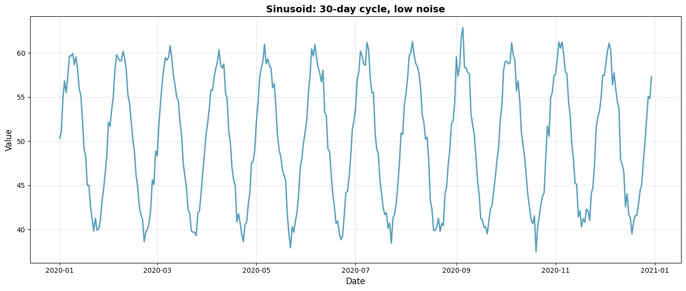

Prepare for GluonTS — The `ListDataset`¶

Before any model can train, your data must be in GluonTS’s ListDataset format. Each entry is a dictionary with:

start — the first timestamp (string or pd.Timestamp)
target — a 1-D array of the values you want to forecast
freq — the time series frequency ("D" for daily, "H" for hourly, "W" for weekly)

Under the hood, this is what GluonTS sees:

from gluonts.dataset.common import ListDataset

train_ds = ListDataset([
    {"start": "2020-01-01", "target": [50.1, 48.3, 52.7, ...]}
], freq="D")

Our prepare_synthetic_dataset utility handles the train/test split and conversion for you. The last prediction_length days become the test set.

Note: Some models (like DeepAR) also support external features via feat_dynamic_real — we’ll cover that in the example notebook with real COVID-19 covariates. For now, we’re keeping it simple: just a target series.

PREDICTION_LENGTH = 30

sin_data = gluonts.prepare_synthetic_dataset(
    sin_df,
    prediction_length=PREDICTION_LENGTH,
)

gluonts.plot_train_test_split(sin_data, title="Sinusoid - Train / Test Split")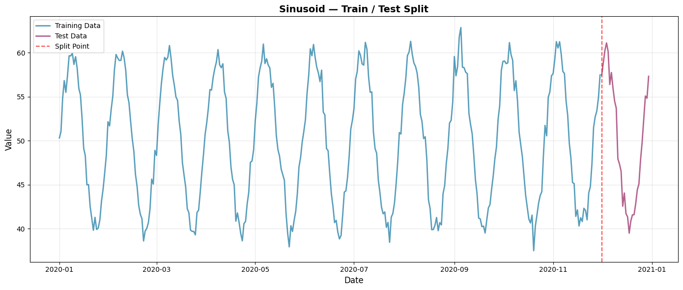


Data split information:
• Training data: 335 points
• Test data: 30 points
• The red line shows where training ends and testing begins

DeepAR on the Sinusoid¶

Analogy: Think of DeepAR like reading a book — it processes the story sequentially, remembering earlier chapters so it can predict what comes next. Technically, it uses a Recurrent Neural Network (RNN) that keeps a hidden state as it moves through your time series.

When to reach for DeepAR¶

Your data has complex patterns — seasonality, multiple waves, trends that shift
Long-term memory matters — what happened weeks ago still influences today
You want to include external features (e.g., mobility data alongside case counts)

Key parameters¶

Parameter	What it controls	Our value
`prediction_length`	How far ahead to forecast	30 days
`context_length`	How far back the model looks (rule of thumb: 2–4× prediction_length)	60 days
`freq`	Data frequency	`"D"` (daily)
`num_layers`	RNN depth — more layers = more capacity	2
`hidden_size`	Neurons per layer	40
`trainer_kwargs`	Training config (epochs, learning rate, etc.)	`{"max_epochs": 5}`

Configure DeepAR¶

deepar_estimator = DeepAREstimator(
    prediction_length=PREDICTION_LENGTH,
    context_length=60,
    freq="D",
    num_layers=2,
    hidden_size=40,
    trainer_kwargs={"max_epochs": 5},
)

Train DeepAR¶

Calling .train() runs the full training loop (powered by PyTorch Lightning).

deepar_predictor = deepar_estimator.train(sin_data["train_ds"])
print("DeepAR training complete")

GPU available: False, used: False
TPU available: False, using: 0 TPU cores
IPU available: False, using: 0 IPUs
HPU available: False, using: 0 HPUs

  | Name  | Type        | Params | In sizes                                                         | Out sizes   
------------------------------------------------------------------------------------------------------------------------
0 | model | DeepARModel | 25.9 K | [[1, 1], [1, 1], [1, 1152, 4], [1, 1152], [1, 1152], [1, 30, 4]] | [1, 100, 30]
------------------------------------------------------------------------------------------------------------------------
25.9 K    Trainable params
0         Non-trainable params
25.9 K    Total params
0.104     Total estimated model params size (MB)

Epoch 0: |                                                  | 50/? [00:03<00:00, 14.66it/s, v_num=4, train_loss=4.160]

Epoch 0, global step 50: 'train_loss' reached 4.16007 (best 4.16007), saving model to '/curr_dir/lightning_logs/version_4/checkpoints/epoch=0-step=50.ckpt' as top 1

Epoch 1: |                                                  | 50/? [00:03<00:00, 15.04it/s, v_num=4, train_loss=2.840]

Epoch 1, global step 100: 'train_loss' reached 2.83587 (best 2.83587), saving model to '/curr_dir/lightning_logs/version_4/checkpoints/epoch=1-step=100.ckpt' as top 1

Epoch 2: |                                                  | 50/? [00:04<00:00, 11.30it/s, v_num=4, train_loss=2.110]

Epoch 2, global step 150: 'train_loss' reached 2.11258 (best 2.11258), saving model to '/curr_dir/lightning_logs/version_4/checkpoints/epoch=2-step=150.ckpt' as top 1

Epoch 3: |                                                  | 50/? [00:03<00:00, 13.25it/s, v_num=4, train_loss=1.940]

Epoch 3, global step 200: 'train_loss' reached 1.93647 (best 1.93647), saving model to '/curr_dir/lightning_logs/version_4/checkpoints/epoch=3-step=200.ckpt' as top 1

Epoch 4: |                                                  | 50/? [00:03<00:00, 15.50it/s, v_num=4, train_loss=1.860]

Epoch 4, global step 250: 'train_loss' reached 1.86255 (best 1.86255), saving model to '/curr_dir/lightning_logs/version_4/checkpoints/epoch=4-step=250.ckpt' as top 1
`Trainer.fit` stopped: `max_epochs=5` reached.

Epoch 4: |                                                  | 50/? [00:03<00:00, 15.47it/s, v_num=4, train_loss=1.860]
DeepAR training complete

Generate Forecasts¶

Unlike traditional models that output a single number per time step, GluonTS models produce probabilistic forecasts — a distribution of possible futures. Here’s what that means in practice:

make_evaluation_predictions(...) generates num_samples possible future trajectories (e.g., 100 different “what-if” scenarios).
From those samples you can extract:
- forecast.mean — the average prediction (point forecast)
- forecast.quantile(0.5) — the median prediction
- forecast.quantile(0.1) / forecast.quantile(0.9) — 80% confidence interval
- forecast.quantile(0.05) / forecast.quantile(0.95) — 90% confidence interval
- forecast.samples — all raw samples, shape (num_samples, prediction_length)

This is powerful because it tells you not just what the model expects, but how confident it is. Wide intervals = high uncertainty; narrow intervals = the model is more sure.

forecast_it, ts_it = make_evaluation_predictions(
    dataset=sin_data["test_ds"],
    predictor=deepar_predictor,
    num_samples=100,
)

deepar_forecasts = list(forecast_it)
deepar_ts = list(ts_it)
deepar_forecast = deepar_forecasts[0]

print(f"Forecast shape: {deepar_forecast.samples.shape}")
print(
    f"  = {deepar_forecast.samples.shape[0]} sample paths, each {deepar_forecast.samples.shape[1]} steps"
)

Forecast shape: (100, 30)
  → 100 sample paths, each 30 steps

Visualize DeepAR on Sinusoid¶

The shaded region shows the 80% confidence interval — the model’s estimate of where the true value is likely to fall.

gluonts.plot_forecast_result(sin_data, deepar_forecast, model_name="DeepAR")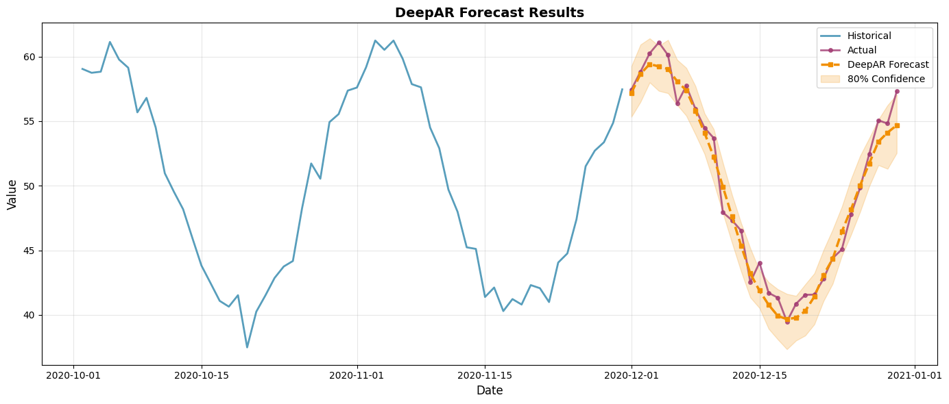


DeepAR forecast summary:
• Blue line shows recent historical data
• Red line shows what actually happened
• Orange dashed line is the model's prediction
• Shaded area shows the model's uncertainty (80% confidence)

Evaluate DeepAR¶

We use three standard metrics to measure forecast quality:

MAE (Mean Absolute Error) — average absolute difference, in original units. Easy to interpret.
RMSE (Root Mean Square Error) — like MAE, but penalizes large errors more heavily.
MAPE (Mean Absolute Percentage Error) — percentage error, so you can compare across different scales.

sin_actuals = sin_data["test_df"]["value"].values
deepar_sin_metrics = gluonts.calculate_metrics(deepar_forecast.mean, sin_actuals)

gluonts.print_metrics(deepar_sin_metrics, model_name="DeepAR on Sinusoid")


📊 DeepAR on Sinusoid Performance Metrics:
============================================================
MAE (Mean Absolute Error):            0.92
RMSE (Root Mean Squared Error):       1.15
MAPE (Mean Abs. %% Error):             1.85 %%
ME (Mean Error / Bias):              -0.45
Maximum Error:                         2.62
============================================================
✅ Excellent! Error less than 10%
⚖️  Low bias - not systematically over/under-predicting

Checkpoint: You just completed the full GluonTS workflow — configure, train, forecast, visualize, evaluate. This is the same 5-step pattern for every GluonTS model. From here on we’ll move faster since you know the drill. What changes is the data (increasing complexity) and the model (different architectures), not the workflow itself.

Level 2: Multi-Frequency — Adding Realism¶

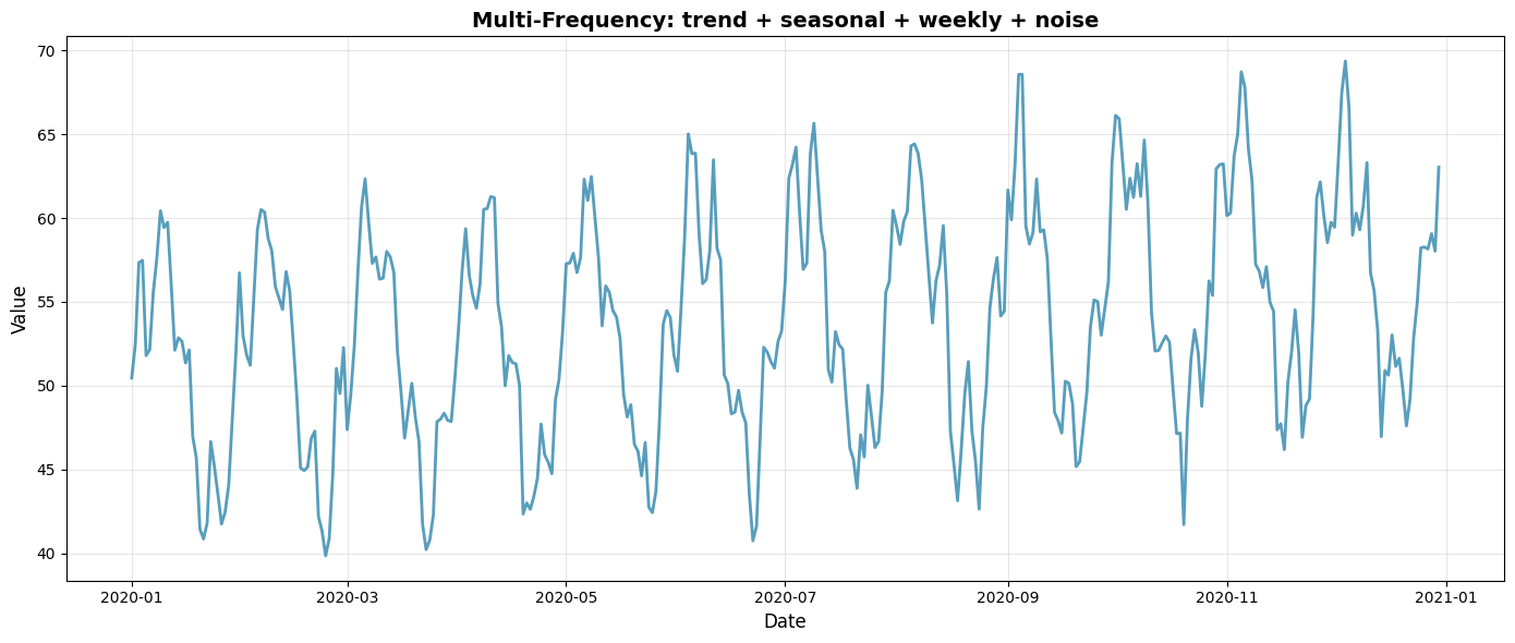
Real time series rarely consist of a single clean cycle. This synthetic series combines four components you’ll encounter in real data:

Linear trend — a slow upward drift over time
30-day seasonal cycle — the dominant pattern (like monthly seasonality)
7-day weekly cycle — a secondary oscillation (like weekend effects)
Gaussian noise — random variation

This is much closer to what you’d see in business metrics, health data, or economic indicators.

Generate and Visualize¶

multi_df = gluonts.generate_multi_frequency(
    n_points=365,
    noise_std=1.5,
    seed=42,
)

gluonts.plot_synthetic_series(
    multi_df, title="Multi-Frequency: trend + seasonal + weekly + noise"
)

multi_data = gluonts.prepare_synthetic_dataset(
    multi_df,
    prediction_length=PREDICTION_LENGTH,
)

gluonts.plot_train_test_split(
    multi_data, title="Multi-Frequency - Train / Test Split"
)


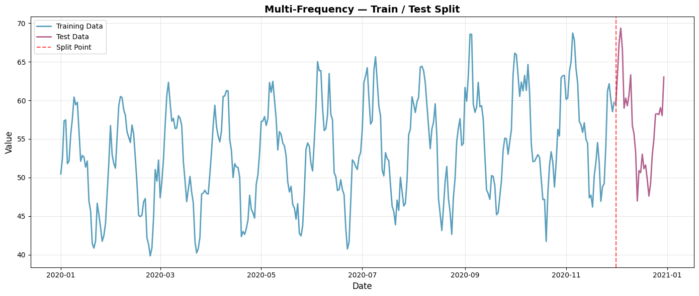
Data split information:
• Training data: 335 points
• Test data: 30 points
• The red line shows where training ends and testing begins

DeepAR on Multi-Frequency¶

We use the same DeepAR configuration. The question is: can it decompose the overlapping cycles and extrapolate the trend?

deepar_multi_est = DeepAREstimator(
    prediction_length=PREDICTION_LENGTH,
    context_length=60,
    freq="D",
    num_layers=2,
    hidden_size=40,
    trainer_kwargs={"max_epochs": 5},
)

deepar_multi_pred = deepar_multi_est.train(multi_data["train_ds"])
print("DeepAR training complete")

GPU available: False, used: False
TPU available: False, using: 0 TPU cores
IPU available: False, using: 0 IPUs
HPU available: False, using: 0 HPUs

  | Name  | Type        | Params | In sizes                                                         | Out sizes   
------------------------------------------------------------------------------------------------------------------------
0 | model | DeepARModel | 25.9 K | [[1, 1], [1, 1], [1, 1152, 4], [1, 1152], [1, 1152], [1, 30, 4]] | [1, 100, 30]
------------------------------------------------------------------------------------------------------------------------
25.9 K    Trainable params
0         Non-trainable params
25.9 K    Total params
0.104     Total estimated model params size (MB)

Epoch 0: |                                                  | 50/? [00:02<00:00, 18.10it/s, v_num=5, train_loss=4.270]

Epoch 0, global step 50: 'train_loss' reached 4.27181 (best 4.27181), saving model to '/curr_dir/lightning_logs/version_5/checkpoints/epoch=0-step=50.ckpt' as top 1

Epoch 1: |                                                  | 50/? [00:02<00:00, 16.92it/s, v_num=5, train_loss=3.020]

Epoch 1, global step 100: 'train_loss' reached 3.01515 (best 3.01515), saving model to '/curr_dir/lightning_logs/version_5/checkpoints/epoch=1-step=100.ckpt' as top 1

Epoch 2: |                                                  | 50/? [00:02<00:00, 17.86it/s, v_num=5, train_loss=2.640]

Epoch 2, global step 150: 'train_loss' reached 2.64275 (best 2.64275), saving model to '/curr_dir/lightning_logs/version_5/checkpoints/epoch=2-step=150.ckpt' as top 1

Epoch 3: |                                                  | 50/? [00:03<00:00, 14.01it/s, v_num=5, train_loss=2.230]

Epoch 3, global step 200: 'train_loss' reached 2.23282 (best 2.23282), saving model to '/curr_dir/lightning_logs/version_5/checkpoints/epoch=3-step=200.ckpt' as top 1

Epoch 4: |                                                  | 50/? [00:02<00:00, 17.21it/s, v_num=5, train_loss=2.120]

Epoch 4, global step 250: 'train_loss' reached 2.11710 (best 2.11710), saving model to '/curr_dir/lightning_logs/version_5/checkpoints/epoch=4-step=250.ckpt' as top 1
`Trainer.fit` stopped: `max_epochs=5` reached.

Epoch 4: |                                                  | 50/? [00:02<00:00, 17.18it/s, v_num=5, train_loss=2.120]
DeepAR training complete

forecast_it, ts_it = make_evaluation_predictions(
    dataset=multi_data["test_ds"],
    predictor=deepar_multi_pred,
    num_samples=100,
)
deepar_multi_fc = list(forecast_it)[0]

gluonts.plot_forecast_result(multi_data, deepar_multi_fc, model_name="DeepAR")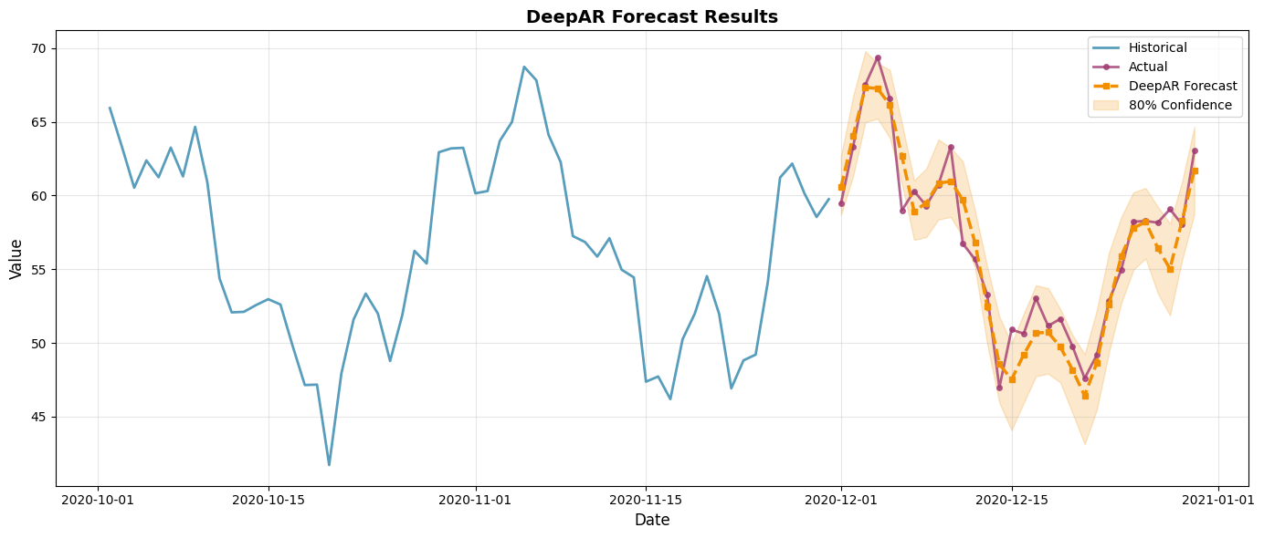


DeepAR forecast summary:
• Blue line shows recent historical data
• Red line shows what actually happened
• Orange dashed line is the model's prediction
• Shaded area shows the model's uncertainty (80% confidence)

multi_actuals = multi_data["test_df"]["value"].values
deepar_multi_metrics = gluonts.calculate_metrics(
    deepar_multi_fc.mean, multi_actuals
)

gluonts.print_metrics(
    deepar_multi_metrics, model_name="DeepAR on Multi-Frequency"
)


📊 DeepAR on Multi-Frequency Performance Metrics:
============================================================
MAE (Mean Absolute Error):            1.35
RMSE (Root Mean Squared Error):       1.73
MAPE (Mean Abs. %% Error):             2.41 %%
ME (Mean Error / Bias):              -0.50
Maximum Error:                         4.05
============================================================
✅ Excellent! Error less than 10%
⚖️  Low bias - not systematically over/under-predicting

SimpleFeedForward on Multi-Frequency¶

Now let’s try a different model on the same data. SimpleFeedForward takes a fixed window of recent history and maps it directly to the future through a basic neural network. No memory of what came before that window — think of it as glancing at the last few pages of a book instead of reading the whole thing.

When to reach for SimpleFeedForward¶

You need fast training — results in seconds, not minutes
Your data has stable, smooth trends without complex seasonality
You want a quick baseline to compare fancier models against

How it differs from DeepAR¶

	DeepAR	SimpleFeedForward
Architecture	RNN (sequential memory)	Feedforward (snapshot)
Hidden layers	`hidden_size` (single int)	`hidden_dimensions` (list of ints)
External features	Supported	Not supported
`freq` parameter	Required	Not accepted
Training speed	Minutes	Seconds

ff_estimator = SimpleFeedForwardEstimator(
    prediction_length=PREDICTION_LENGTH,
    context_length=60,
    hidden_dimensions=[40, 40],
    trainer_kwargs={"max_epochs": 5},
)

ff_predictor = ff_estimator.train(multi_data["train_ds"])
print("SimpleFeedForward training complete")

GPU available: False, used: False
TPU available: False, using: 0 TPU cores
IPU available: False, using: 0 IPUs
HPU available: False, using: 0 HPUs

  | Name  | Type                   | Params
-------------------------------------------------
0 | model | SimpleFeedForwardModel | 51.8 K
-------------------------------------------------
51.8 K    Trainable params
0         Non-trainable params
51.8 K    Total params
0.207     Total estimated model params size (MB)

Epoch 0: |                                                 | 50/? [00:00<00:00, 192.74it/s, v_num=6, train_loss=4.740]

Epoch 0, global step 50: 'train_loss' reached 4.74095 (best 4.74095), saving model to '/curr_dir/lightning_logs/version_6/checkpoints/epoch=0-step=50.ckpt' as top 1

Epoch 1: |                                                 | 50/? [00:00<00:00, 169.52it/s, v_num=6, train_loss=3.480]

Epoch 1, global step 100: 'train_loss' reached 3.48431 (best 3.48431), saving model to '/curr_dir/lightning_logs/version_6/checkpoints/epoch=1-step=100.ckpt' as top 1

Epoch 2: |                                                 | 50/? [00:00<00:00, 161.82it/s, v_num=6, train_loss=3.010]

Epoch 2, global step 150: 'train_loss' reached 3.00814 (best 3.00814), saving model to '/curr_dir/lightning_logs/version_6/checkpoints/epoch=2-step=150.ckpt' as top 1

Epoch 3: |                                                 | 50/? [00:00<00:00, 179.39it/s, v_num=6, train_loss=2.760]

Epoch 3, global step 200: 'train_loss' reached 2.75951 (best 2.75951), saving model to '/curr_dir/lightning_logs/version_6/checkpoints/epoch=3-step=200.ckpt' as top 1

Epoch 4: |                                                 | 50/? [00:00<00:00, 200.33it/s, v_num=6, train_loss=2.740]

Epoch 4, global step 250: 'train_loss' reached 2.73679 (best 2.73679), saving model to '/curr_dir/lightning_logs/version_6/checkpoints/epoch=4-step=250.ckpt' as top 1
`Trainer.fit` stopped: `max_epochs=5` reached.

Epoch 4: |                                                 | 50/? [00:00<00:00, 196.35it/s, v_num=6, train_loss=2.740]
SimpleFeedForward training complete

forecast_it, ts_it = make_evaluation_predictions(
    dataset=multi_data["test_ds"],
    predictor=ff_predictor,
    num_samples=100,
)
ff_multi_fc = list(forecast_it)[0]

gluonts.plot_forecast_result(
    multi_data, ff_multi_fc, model_name="SimpleFeedForward"
)


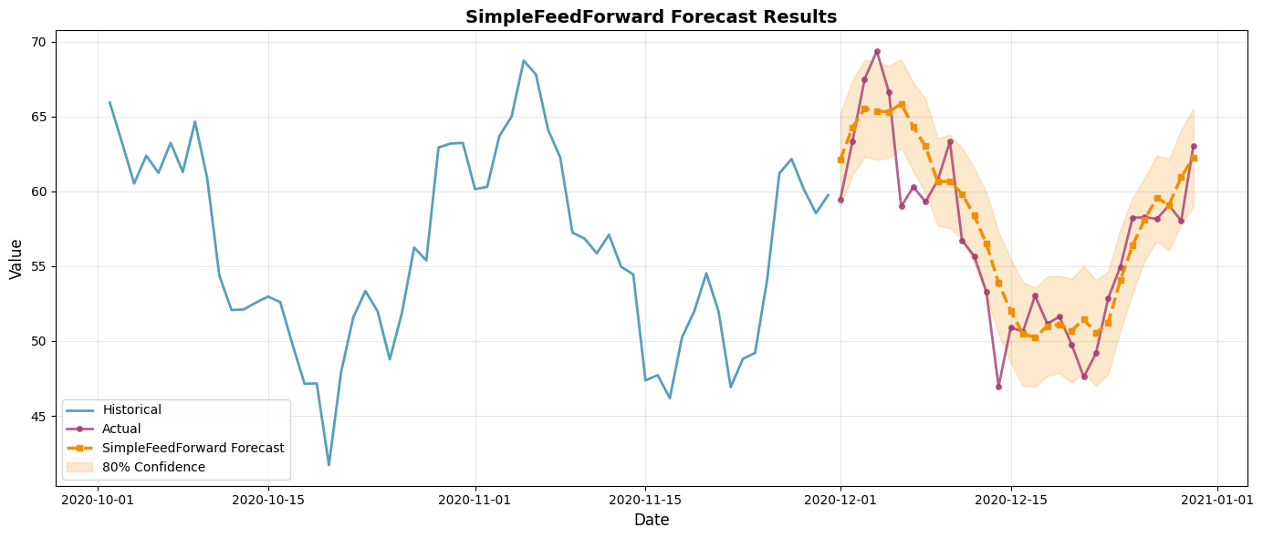
SimpleFeedForward forecast summary:
• Blue line shows recent historical data
• Red line shows what actually happened
• Orange dashed line is the model's prediction
• Shaded area shows the model's uncertainty (80% confidence)

ff_multi_metrics = gluonts.calculate_metrics(ff_multi_fc.mean, multi_actuals)

gluonts.print_metrics(
    ff_multi_metrics, model_name="SimpleFeedForward on Multi-Frequency"
)


📊 SimpleFeedForward on Multi-Frequency Performance Metrics:
============================================================
MAE (Mean Absolute Error):            2.15
RMSE (Root Mean Squared Error):       2.79
MAPE (Mean Abs. %% Error):             3.84 %%
ME (Mean Error / Bias):               0.89
Maximum Error:                         6.91
============================================================
✅ Excellent! Error less than 10%
⚖️  Low bias - not systematically over/under-predicting

Level 3: Regime Change — The Hard Problem¶

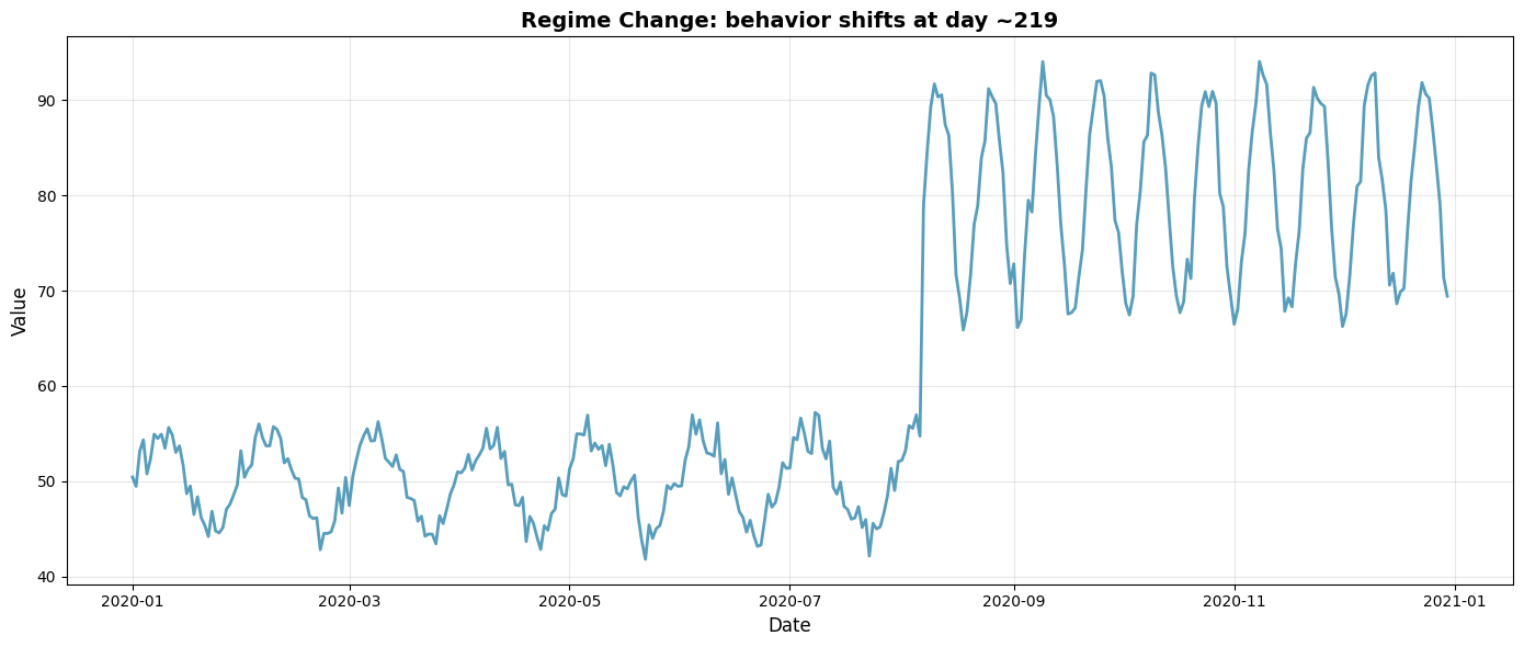
This is where things get interesting. The series behaves one way for the first half, then abruptly shifts to a different baseline, amplitude, and frequency.

Think of real-world analogs:

A new COVID variant causing a sudden surge
A product going viral and changing demand patterns
A policy change shifting economic indicators

Most models struggle here because their training data comes from the old regime, but they need to forecast in the new one.

Generate and Visualize¶

regime_df = gluonts.generate_regime_change(
    n_points=365,
    changepoint_frac=0.6,
    noise_std=1.5,
    seed=42,
)

gluonts.plot_synthetic_series(
    regime_df, title="Regime Change: behavior shifts at day ~219"
)

regime_data = gluonts.prepare_synthetic_dataset(
    regime_df,
    prediction_length=PREDICTION_LENGTH,
)

gluonts.plot_train_test_split(
    regime_data, title="Regime Change - Train / Test Split"
)


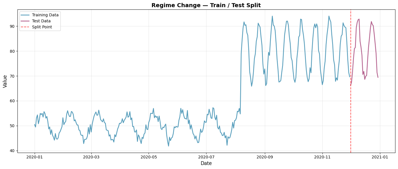
Data split information:
• Training data: 335 points
• Test data: 30 points
• The red line shows where training ends and testing begins

DeepNPTS on Regime Change¶

DeepAR and SimpleFeedForward assume the future follows a known shape (like a bell curve). DeepNPTS says “I’ll figure out the shape from the data itself.” It’s non-parametric — it learns the distribution directly without assuming normal, Poisson, or any other family.

This makes it especially powerful when your data doesn’t behave “normally” — sudden regime shifts, heavy tails, or distributions that change over time.

When to reach for DeepNPTS¶

The distribution changes over time (e.g., calm periods vs. surges)
You expect regime shifts — the data behaves differently before and after some event
Your data has unusual shapes — heavy tails, multi-modal, skewed

How it differs from DeepAR¶

	DeepAR	DeepNPTS
Distribution	Parametric (assumes Gaussian)	Non-parametric (learned from data)
Epochs config	`trainer_kwargs={"max_epochs": N}`	`epochs=N` (direct parameter)
Hidden layers	`hidden_size` (single int)	`num_hidden_nodes` (list of ints)
Regime shifts	Can struggle	Designed for this

Watch the code below — notice the two API quirks: epochs is a direct parameter (not inside trainer_kwargs), and the hidden layer parameter is called num_hidden_nodes instead of hidden_size.

npts_estimator = DeepNPTSEstimator(
    prediction_length=PREDICTION_LENGTH,
    context_length=60,
    freq="D",
    num_hidden_nodes=[40, 40],
    epochs=5,
)

npts_predictor = npts_estimator.train(regime_data["train_ds"])
print("DeepNPTS training complete")

Loss for epoch 0: 2.505797874927521
Loss for epoch 1: 2.2752446341514587
Loss for epoch 2: 2.2304137551784518
Loss for epoch 3: 2.175221121311188
Loss for epoch 4: 1.985428268313408
Best loss: 1.985428268313408
DeepNPTS training complete

forecast_it, ts_it = make_evaluation_predictions(
    dataset=regime_data["test_ds"],
    predictor=npts_predictor,
    num_samples=100,
)
npts_regime_fc = list(forecast_it)[0]

gluonts.plot_forecast_result(regime_data, npts_regime_fc, model_name="DeepNPTS")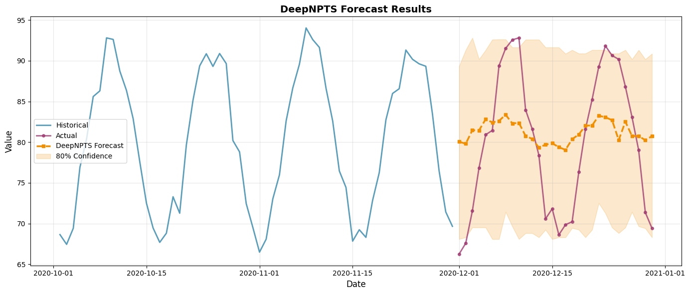


DeepNPTS forecast summary:
• Blue line shows recent historical data
• Red line shows what actually happened
• Orange dashed line is the model's prediction
• Shaded area shows the model's uncertainty (80% confidence)

regime_actuals = regime_data["test_df"]["value"].values
npts_regime_metrics = gluonts.calculate_metrics(
    npts_regime_fc.mean, regime_actuals
)

print("DeepNPTS on Regime Change")
print("=" * 40)
print(f"  MAE:  {npts_regime_metrics['mae']:.2f}")
print(f"  RMSE: {npts_regime_metrics['rmse']:.2f}")
print(f"  MAPE: {npts_regime_metrics['mape']:.2f}%")

DeepNPTS on Regime Change
========================================
  MAE:  6.70
  RMSE: 7.73
  MAPE: 8.67%

DeepAR on Regime Change (Contrast)¶

Let’s run DeepAR on the same regime-change data to see how it compares. Because DeepAR assumes a parametric distribution learned from the full training set, it may struggle with the post-shift behavior.

deepar_regime_est = DeepAREstimator(
    prediction_length=PREDICTION_LENGTH,
    context_length=60,
    freq="D",
    num_layers=2,
    hidden_size=40,
    trainer_kwargs={"max_epochs": 5},
)

deepar_regime_pred = deepar_regime_est.train(regime_data["train_ds"])

forecast_it, ts_it = make_evaluation_predictions(
    dataset=regime_data["test_ds"],
    predictor=deepar_regime_pred,
    num_samples=100,
)
deepar_regime_fc = list(forecast_it)[0]

gluonts.plot_forecast_result(regime_data, deepar_regime_fc, model_name="DeepAR")

GPU available: False, used: False
TPU available: False, using: 0 TPU cores
IPU available: False, using: 0 IPUs
HPU available: False, using: 0 HPUs

  | Name  | Type        | Params | In sizes                                                         | Out sizes   
------------------------------------------------------------------------------------------------------------------------
0 | model | DeepARModel | 25.9 K | [[1, 1], [1, 1], [1, 1152, 4], [1, 1152], [1, 1152], [1, 30, 4]] | [1, 100, 30]
------------------------------------------------------------------------------------------------------------------------
25.9 K    Trainable params
0         Non-trainable params
25.9 K    Total params
0.104     Total estimated model params size (MB)

Epoch 0: |                                                  | 50/? [00:02<00:00, 16.88it/s, v_num=7, train_loss=4.110]

Epoch 0, global step 50: 'train_loss' reached 4.10991 (best 4.10991), saving model to '/curr_dir/lightning_logs/version_7/checkpoints/epoch=0-step=50.ckpt' as top 1

Epoch 1: |                                                  | 50/? [00:02<00:00, 17.95it/s, v_num=7, train_loss=3.150]

Epoch 1, global step 100: 'train_loss' reached 3.15040 (best 3.15040), saving model to '/curr_dir/lightning_logs/version_7/checkpoints/epoch=1-step=100.ckpt' as top 1

Epoch 2: |                                                  | 50/? [00:02<00:00, 17.69it/s, v_num=7, train_loss=2.820]

Epoch 2, global step 150: 'train_loss' reached 2.82018 (best 2.82018), saving model to '/curr_dir/lightning_logs/version_7/checkpoints/epoch=2-step=150.ckpt' as top 1

Epoch 3: |                                                  | 50/? [00:02<00:00, 16.96it/s, v_num=7, train_loss=2.660]

Epoch 3, global step 200: 'train_loss' reached 2.65559 (best 2.65559), saving model to '/curr_dir/lightning_logs/version_7/checkpoints/epoch=3-step=200.ckpt' as top 1

Epoch 4: |                                                  | 50/? [00:02<00:00, 16.76it/s, v_num=7, train_loss=2.520]

Epoch 4, global step 250: 'train_loss' reached 2.52409 (best 2.52409), saving model to '/curr_dir/lightning_logs/version_7/checkpoints/epoch=4-step=250.ckpt' as top 1
`Trainer.fit` stopped: `max_epochs=5` reached.

Epoch 4: |                                                  | 50/? [00:02<00:00, 16.72it/s, v_num=7, train_loss=2.520]


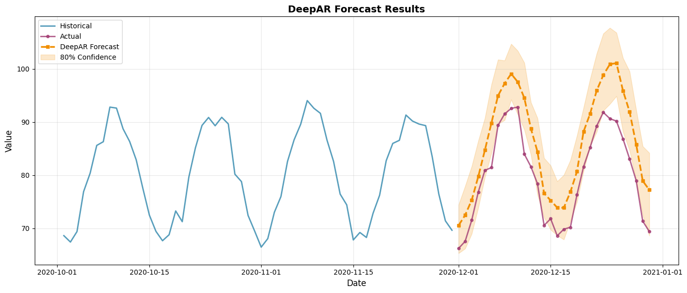
DeepAR forecast summary:
• Blue line shows recent historical data
• Red line shows what actually happened
• Orange dashed line is the model's prediction
• Shaded area shows the model's uncertainty (80% confidence)

deepar_regime_metrics = gluonts.calculate_metrics(
    deepar_regime_fc.mean, regime_actuals
)

print("DeepAR on Regime Change")
print("=" * 40)
print(f"  MAE:  {deepar_regime_metrics['mae']:.2f}")
print(f"  RMSE: {deepar_regime_metrics['rmse']:.2f}")
print(f"  MAPE: {deepar_regime_metrics['mape']:.2f}%")

DeepAR on Regime Change
========================================
  MAE:  6.40
  RMSE: 6.73
  MAPE: 7.96%

Model Comparison¶

Let’s bring all results together. Each model was tested on the data type that best highlights its strengths and weaknesses.

import pandas as pd

comparison = pd.DataFrame(
    {
        "Model": [
            "DeepAR (sinusoid)",
            "DeepAR (multi-freq)",
            "SimpleFeedForward (multi-freq)",
            "DeepNPTS (regime change)",
            "DeepAR (regime change)",
        ],
        "MAE": [
            deepar_sin_metrics["mae"],
            deepar_multi_metrics["mae"],
            ff_multi_metrics["mae"],
            npts_regime_metrics["mae"],
            deepar_regime_metrics["mae"],
        ],
        "RMSE": [
            deepar_sin_metrics["rmse"],
            deepar_multi_metrics["rmse"],
            ff_multi_metrics["rmse"],
            npts_regime_metrics["rmse"],
            deepar_regime_metrics["rmse"],
        ],
        "MAPE (%)": [
            deepar_sin_metrics["mape"],
            deepar_multi_metrics["mape"],
            ff_multi_metrics["mape"],
            npts_regime_metrics["mape"],
            deepar_regime_metrics["mape"],
        ],
    }
)

print(comparison.to_string(index=False, float_format="%.2f"))

                         Model  MAE  RMSE  MAPE (%)
             DeepAR (sinusoid) 0.92  1.15      1.85
           DeepAR (multi-freq) 1.35  1.73      2.41
SimpleFeedForward (multi-freq) 2.15  2.79      3.84
      DeepNPTS (regime change) 6.70  7.73      8.67
        DeepAR (regime change) 6.40  6.73      7.96

Summary¶

What You Learned¶

Data preparation — GluonTS uses ListDataset with start, target, and optional feat_dynamic_real
Three models — DeepAR (RNN, complex patterns), SimpleFeedForward (fast baseline), DeepNPTS (flexible, non-parametric)
One workflow — estimator.train() then make_evaluation_predictions() — same pattern for every model
Probabilistic output — every forecast gives you means, medians, quantiles, and raw samples
Model choice matters — the right model depends on your data’s characteristics

Which Model Should You Choose?¶

If your data has...	Try this model	Why
Complex seasonality, multiple waves	DeepAR	RNN captures long-range dependencies
Stable trends, need fast results	SimpleFeedForward	Trains in seconds, good baseline
Regime shifts, unusual distributions	DeepNPTS	Non-parametric — adapts to changing behavior
No idea yet	Start with SimpleFeedForward	Fast to test, then try DeepAR for more accuracy

Quick Reference¶

Task	Code
Point forecast (mean)	`forecast.mean`
Median forecast	`forecast.quantile(0.5)`
80% confidence interval	`forecast.quantile(0.1)` to `forecast.quantile(0.9)`
Raw sample paths	`forecast.samples` (shape: `num_samples × prediction_length`)

Tips for Better Results¶

Area	Tip
Context length	Start at 2× your `prediction_length`, try 3× and 4×
Epochs	5–10 for experiments, 20–30 for final models
Features	More isn’t always better — test with and without
Data quality	Handle missing values and normalize if needed

Troubleshooting¶

Problem	Fix
“Wrong number of features”	`num_feat_dynamic_real` must match the rows in your `feat_dynamic_real` array
Training too slow	Reduce epochs, shrink `context_length`, or use SimpleFeedForward
Poor forecast quality	Increase `context_length`, train longer, or try DeepNPTS for regime changes
“Unexpected keyword argument”	DeepAR: `trainer_kwargs={"max_epochs": N}`. DeepNPTS: `epochs=N`. SimpleFeedForward: no `freq` parameter

Resources¶

GluonTS Documentation · GitHub · PyTorch Lightning

What’s Next?¶

Now that you understand how GluonTS works on clean synthetic data, move to GluonTS.example.ipynb to see these same models applied to real COVID-19 case prediction — with feature engineering, multiple covariates, scenario analysis, and all the messiness of real-world data.

GluonTS API Tutorial: Probabilistic Time Series Forecasting

Prerequisites¶

What You’ll Learn¶

The Three Models¶

Why Synthetic Data?¶

Setup¶

The GluonTS Workflow¶

Level 1: Sinusoid — The Simplest Pattern¶

Generate and Visualize the Sinusoid¶

Prepare for GluonTS — The ListDataset¶

DeepAR on the Sinusoid¶

When to reach for DeepAR¶

Key parameters¶

Configure DeepAR¶

Train DeepAR¶

Generate Forecasts¶

Visualize DeepAR on Sinusoid¶

Evaluate DeepAR¶

Level 2: Multi-Frequency — Adding Realism¶

Generate and Visualize¶

DeepAR on Multi-Frequency¶

SimpleFeedForward on Multi-Frequency¶

When to reach for SimpleFeedForward¶

How it differs from DeepAR¶

Level 3: Regime Change — The Hard Problem¶

Generate and Visualize¶

DeepNPTS on Regime Change¶

When to reach for DeepNPTS¶

How it differs from DeepAR¶

DeepAR on Regime Change (Contrast)¶

Model Comparison¶

Summary¶

What You Learned¶

Which Model Should You Choose?¶

Quick Reference¶

Tips for Better Results¶

Troubleshooting¶

Resources¶

What’s Next?¶

Prepare for GluonTS — The `ListDataset`¶