TensorFlow: Structural Time Series Forecasting
This notebook demonstrates a complete end-to-end time series forecasting pipeline using TensorFlow Probability’s Structural Time Series (STS) module.
Workflow:
- Generate a synthetic daily time series with trend, seasonality, holidays, and autoregressive noise
- Build an STS model combining multiple interpretable components
- Fit the model via Variational Inference (VI)
- Forecast future values and evaluate performance
%load_ext autoreload
%autoreload 2
%matplotlib inline

import logging

import matplotlib.pyplot as plt
import numpy as np
import scipy.stats as stats
import sklearn.metrics as metrics
import tensorflow_probability as tfp
import tf_keras

import tensorflow_utils as tteteuti

_LOG = logging.getLogger(__name__)
2026-03-10 16:28:44.100240: I external/local_xla/xla/tsl/cuda/cudart_stub.cc:31] Could not find cuda drivers on your machine, GPU will not be used.
2026-03-10 16:28:44.100451: I tensorflow/core/util/port.cc:153] oneDNN custom operations are on. You may see slightly different numerical results due to floating-point round-off errors from different computation orders. To turn them off, set the environment variable `TF_ENABLE_ONEDNN_OPTS=0`.
2026-03-10 16:28:44.137759: I tensorflow/core/platform/cpu_feature_guard.cc:210] This TensorFlow binary is optimized to use available CPU instructions in performance-critical operations.
To enable the following instructions: AVX2 AVX_VNNI FMA, in other operations, rebuild TensorFlow with the appropriate compiler flags.
2026-03-10 16:28:45.032141: I tensorflow/core/util/port.cc:153] oneDNN custom operations are on. You may see slightly different numerical results due to floating-point round-off errors from different computation orders. To turn them off, set the environment variable `TF_ENABLE_ONEDNN_OPTS=0`.
2026-03-10 16:28:45.032394: I external/local_xla/xla/tsl/cuda/cudart_stub.cc:31] Could not find cuda drivers on your machine, GPU will not be used.
Config
All model and data parameters are centralised here so the notebook can be reproduced by changing a single dictionary.
config = {
    # Train / test split.
    "train_start_date": "2020-01-01",
    "train_end_date": "2023-12-31",
    "test_start_date": "2024-01-01",
    "test_end_date": "2024-12-31",
    "data": {
        # Linear trend.
        "slope": 0.005,
        "intercept": 15,
        # Weekly seasonal drift.
        "seasonal_drift_scale": 0.5,
        # Holiday dates and their additive impact.
        "holidays_dates": [
            "2020-12-25",
            "2021-12-25",
            "2022-12-25",
            "2023-12-25",
            "2024-12-25",
        ],
        "holidays_impact": 0.25,
        # AR(1) coefficient.
        "ar_order": 1,
        "phi": 0.7,
        # Observation noise.
        "seed": 42,
        "observational_noise_sigma": 2.0,
    },
    "model": {
        # Weekly seasonality: 7 seasons, 1 step each.
        "num_seasons": 7,
        "num_steps_per_season": 1,
        "learning_rate": 0.1,
        # Number of VI optimisation steps.
        "num_steps": 200,
    },
}
print(config)
{'train_start_date': '2020-01-01', 'train_end_date': '2023-12-31', 'test_start_date': '2024-01-01', 'test_end_date': '2024-12-31', 'data': {'slope': 0.005, 'intercept': 15, 'seasonal_drift_scale': 0.5, 'holidays_dates': ['2020-12-25', '2021-12-25', '2022-12-25', '2023-12-25', '2024-12-25'], 'holidays_impact': 0.25, 'ar_order': 1, 'phi': 0.7, 'seed': 42, 'observational_noise_sigma': 2.0}, 'model': {'num_seasons': 7, 'num_steps_per_season': 1, 'learning_rate': 0.1, 'num_steps': 200}}
Part 1: Data Generation
We generate a realistic synthetic daily time series that combines:
- A linear trend (slow upward drift)
- Weekly seasonality with stochastic drift
- Holiday effects (additive spikes on Christmas each year)
- AR(1) autoregression to capture temporal dependence
- Gaussian observation noise
Using synthetic data lets us later verify that the model recovers the known ground-truth parameters.
df = tteteuti.generate_time_series_data(config)
_LOG.info(tteteuti.df_to_str_simple(df))
df.set_index("ds")["y"].plot(
title="Synthetic Daily Time Series",
ylabel="Target variable",
xlabel="Date",
figsize=(12, 4),
)<Axes: title={'center': 'Synthetic Daily Time Series'}, xlabel='Date', ylabel='Target variable'>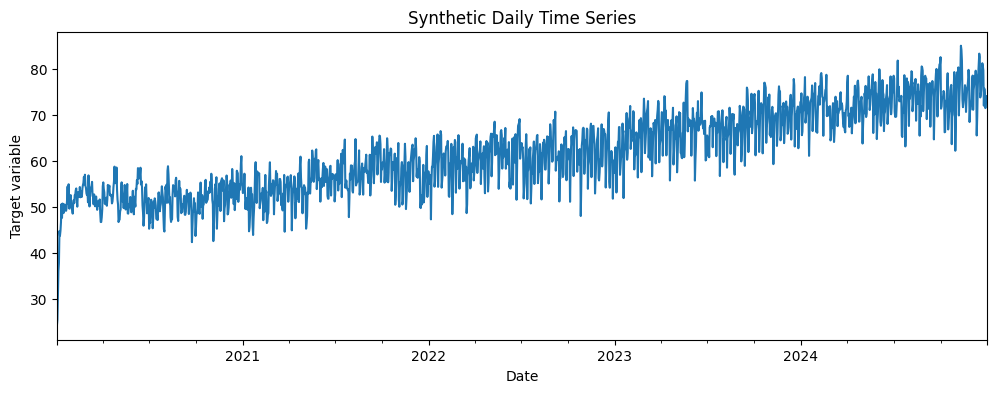
# Split into train and test sets.
train_mask = (df["ds"] >= config["train_start_date"]) & (
    df["ds"] <= config["train_end_date"]
)
test_mask = (df["ds"] >= config["test_start_date"]) & (
    df["ds"] <= config["test_end_date"]
)
df_train = df[train_mask].reset_index(drop=True)
df_test = df[test_mask].reset_index(drop=True)
_LOG.info("Train rows=%d, Test rows=%d", len(df_train), len(df_test))
Part 2: Model Building
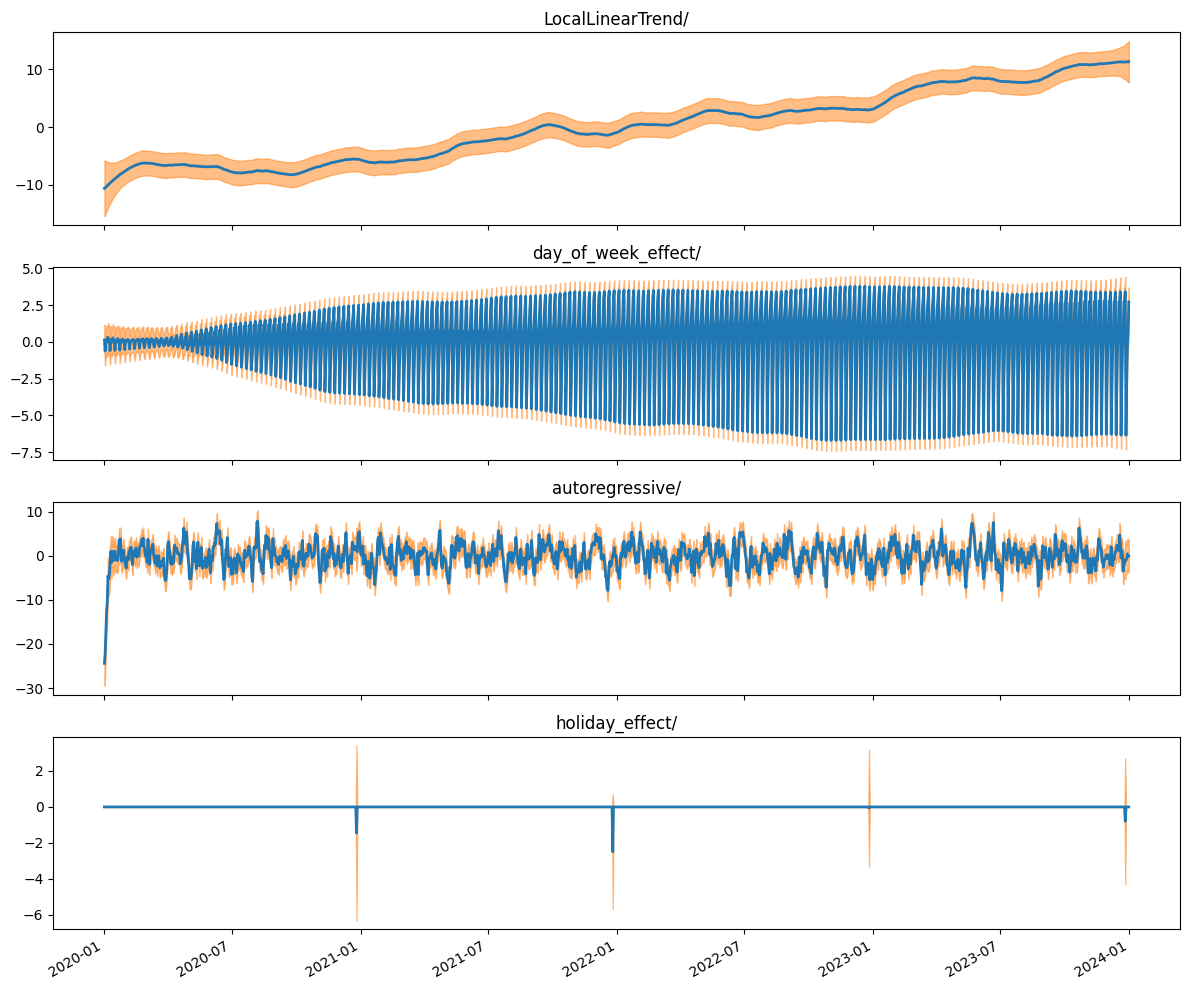
The STS model decomposes the observed series into four interpretable components:
| Component | Purpose |
|---|---|
LocalLinearTrend | Captures slow-moving level and slope |
Seasonal (7 seasons) | Weekly day-of-week effects |
Autoregressive (AR-1) | Short-term temporal dependence |
LinearRegression | Additive holiday spikes |
The components are summed into a tfp.sts.Sum model.
# Build one-hot holiday indicator matrix for the full date range.
holiday_indicators = tteteuti.build_holiday_indicators(config)
_LOG.info("holiday_indicators shape=%s", holiday_indicators.shape)
model = tteteuti.build_sts_model(
df_train["y"].to_numpy(), holiday_indicators, config
)2026-03-10 16:28:45.987563: E external/local_xla/xla/stream_executor/cuda/cuda_platform.cc:51] failed call to cuInit: INTERNAL: CUDA error: Failed call to cuInit: UNKNOWN ERROR (303)
Variational Inference
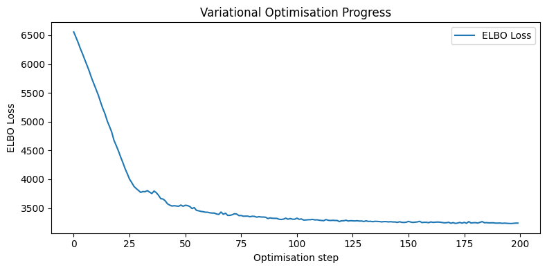
We approximate the posterior over model parameters using Variational Inference (VI):
- Define a factored surrogate posterior
q(θ)(one Normal per parameter) - Maximise the ELBO:
ELBO = E_q[log p(y, θ)] - KL(q || prior) - Use the Adam optimiser for gradient-based optimisation
# Build the variational surrogate posteriors.
variational_posteriors = tfp.sts.build_factored_surrogate_posterior(model=model)
elbo_loss_curve = tfp.vi.fit_surrogate_posterior(
target_log_prob_fn=model.joint_distribution(
observed_time_series=df_train["y"].to_numpy()
).log_prob,
surrogate_posterior=variational_posteriors,
optimizer=tf_keras.optimizers.Adam(
learning_rate=config["model"]["learning_rate"]
),
num_steps=config["model"]["num_steps"],
jit_compile=True,
)
plt.figure(figsize=(8, 4))
plt.plot(elbo_loss_curve, label="ELBO Loss")
plt.xlabel("Optimisation step")
plt.ylabel("ELBO Loss")
plt.title("Variational Optimisation Progress")
plt.legend()
plt.tight_layout()2026-03-10 16:28:56.234079: I external/local_xla/xla/service/service.cc:163] XLA service 0x5f6172061690 initialized for platform Host (this does not guarantee that XLA will be used). Devices:
2026-03-10 16:28:56.234093: I external/local_xla/xla/service/service.cc:171] StreamExecutor device (0): Host, Default Version
2026-03-10 16:28:56.419096: W tensorflow/compiler/tf2xla/kernels/random_ops.cc:108] Warning: Using tf.random.uniform with XLA compilation will ignore seeds; consider using tf.random.stateless_uniform instead if reproducible behavior is desired. fit_surrogate_posterior/StatefulPartitionedCall/monte_carlo_variational_loss/split_seed/sanitize_seed/seed
2026-03-10 16:28:56.433183: I tensorflow/compiler/mlir/tensorflow/utils/dump_mlir_util.cc:269] disabling MLIR crash reproducer, set env var `MLIR_CRASH_REPRODUCER_DIRECTORY` to enable.
WARNING: All log messages before absl::InitializeLog() is called are written to STDERR
I0000 00:00:1773160141.177601     216 device_compiler.h:196] Compiled cluster using XLA!  This line is logged at most once for the lifetime of the process.
# Draw posterior samples.
q_samples_ = variational_posteriors.sample(50)
# Report inferred parameter values.
_LOG.info("Inferred parameters:")
for param in model.parameters:
_LOG.info(
" %s: %.4f ± %.4f",
param.name,
np.mean(q_samples_[param.name], axis=0),
np.std(q_samples_[param.name], axis=0),
)Part 3: Forecasting and Evaluation
With the fitted posterior we:
- Decompose the training signal into its constituent components
- Forecast
num_steps_forecaststeps into the future - Evaluate using MAE and MSE
# Decompose training data into components.
component_dists = tfp.sts.decompose_by_component(
    model,
    observed_time_series=df_train["y"].to_numpy(),
    parameter_samples=q_samples_,
)
component_means_ = {k.name: c.mean() for k, c in component_dists.items()}
component_stddevs_ = {k.name: c.stddev() for k, c in component_dists.items()}
_ = tteteuti.plot_components(
df_train["ds"], component_means_, component_stddevs_
)
# Forecast the test period.
forecast_dist = tfp.sts.forecast(
    model=model,
    observed_time_series=df_train["y"].to_numpy(),
    parameter_samples=q_samples_,
    num_steps_forecast=len(df_test),
)
num_samples = 10
forecast_mean = forecast_dist.mean().numpy()[..., 0]
forecast_scale = forecast_dist.stddev().numpy()[..., 0]
forecast_samples = forecast_dist.sample(num_samples).numpy()[..., 0]
2026-03-10 16:29:09.191232: E tensorflow/core/util/util.cc:131] oneDNN supports DT_INT32 only on platforms with AVX-512. Falling back to the default Eigen-based implementation if present.
fig, ax = tteteuti.plot_forecast(
    df_test["ds"],
    df_test["y"].to_numpy(),
    forecast_mean,
    forecast_scale,
    forecast_samples,
    title="STS Forecast vs Ground Truth",
)
fig.tight_layout()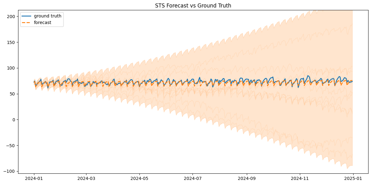
# Residual analysis.
residuals = df_test["y"].to_numpy() - forecast_mean
fig, axes = plt.subplots(1, 2, figsize=(14, 5))
axes[0].plot(df_test["ds"], residuals, color="steelblue")
axes[0].axhline(0, color="red", ls="--")
axes[0].set_title("Residuals Over Time")
axes[0].set_xlabel("Date")
axes[0].set_ylabel("Residual")
stats.probplot(residuals, dist="norm", plot=axes[1])
axes[1].set_title("Q-Q Plot of Residuals")
plt.tight_layout()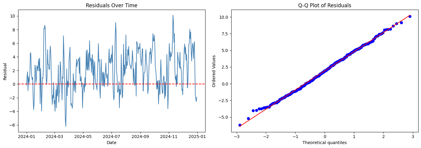
# Performance metrics.
mae = metrics.mean_absolute_error(df_test["y"].to_numpy(), forecast_mean)
mse = metrics.mean_squared_error(df_test["y"].to_numpy(), forecast_mean)
_LOG.info("MAE=%.4f", mae)
_LOG.info("MSE=%.4f", mse)