The 4x3 Grid World: From MDPs to Reinforcement Learning

This notebook teaches sequential decision making through the canonical AIMA 4x3 grid world, built entirely from scratch with numpy (no gymnasium)
The grid world is the unifying example throughout:
- It appears in the MDP definition, utility of states, Bellman equations, value iteration, policy iteration, and Q-learning
The pedagogical arc is:
- Build the environment (states, stochastic transitions, rewards)
- Solve it with full knowledge (value iteration, policy iteration)
- Learn it without knowing the model (Q-learning)

Gridworld 4x3¶

Imports¶

%load_ext autoreload
%autoreload 2

# System libraries.
import logging

# Third-party libraries.
import matplotlib.pyplot as plt
import numpy as np
import seaborn as sns

# Set plotting style.
sns.set_style("whitegrid")
plt.rcParams["figure.figsize"] = (12, 6)

The autoreload extension is already loaded. To reload it, use:
  %reload_ext autoreload

import helpers.hnotebook as hnotebook

import L12_01_gridworld_4x3_utils as utils

# Initialize notebook configuration and logging.
hnotebook.config_notebook()
_LOG = logging.getLogger(__name__)
utils.init_loggers(_LOG)

WARNING: Logger already initialized: skipping

Part 1: Building the Grid World Environment¶

Cell 0: GridWorld API Overview¶

Goal:

See the GridWorld class in action
Build intuition for the environment’s basic structure

The GridWorld class implements the canonical AIMA 4x3 grid world MDP. Key properties accessible from any GridWorld instance:

.states — all 11 reachable cells (col, row) 1-indexed
.actions — the four directions: Up, Down, Left, Right
.terminals — cells that end the episode with a reward
.walls — cells the agent cannot occupy
.transitions(s, a) — the stochastic next-state distribution
.q_value(s, a, u) — expected return of action a under utilities u
.reward(s) — reward collected on entering cell s
.sample_next(s, a, rng) — draw one next state from the model (used by Q-learning)

# Read the code for `GridWorld`.
# ??utils.GridWorld.__init__

# Create the default grid world and inspect its basic properties.
env = utils.GridWorld()
print("env.states (%d):" % len(env.states), env.states)
print("env.actions:", env.actions)
print("env.terminals:", env.terminals)
print("env.walls:", env.walls)
print("env.start:", env.start)
print("env.r_step:", env.r_step)
print("env.gamma:", env.gamma)
print("env.p_intended:", env.p_intended)
print()
print("Each state's reward:")
for s in env.states:
    print("  R(%s) = %.2f" % (s, env.reward(s)))

env.states (11): [(1, 1), (2, 1), (3, 1), (4, 1), (1, 2), (3, 2), (4, 2), (1, 3), (2, 3), (3, 3), (4, 3)]
env.actions: ['Up', 'Down', 'Left', 'Right']
env.terminals: {(4, 3): 1.0, (4, 2): -1.0}
env.walls: {(2, 2)}
env.start: (1, 1)
env.r_step: -0.04
env.gamma: 1.0
env.p_intended: 0.8

Each state's reward:
  R((1, 1)) = -0.04
  R((2, 1)) = -0.04
  R((3, 1)) = -0.04
  R((4, 1)) = -0.04
  R((1, 2)) = -0.04
  R((3, 2)) = -0.04
  R((4, 2)) = -1.00
  R((1, 3)) = -0.04
  R((2, 3)) = -0.04
  R((3, 3)) = -0.04
  R((4, 3)) = 1.00

# Query the transition model for a state-action pair.
env = utils.GridWorld()
s = (1, 1)  # START
a = "Up"
dist = env.transitions(s, a)
print("Pr(s' | s=%s, a=%s):" % (s, a))
for s2, prob in sorted(dist.items(), key=lambda x: -x[1]):
    print(
        "  s' = %s  p = %.2f  arrival reward = %.2f" % (s2, prob, env.reward(s2))
    )
print()
# Sample from the model.
rng = np.random.RandomState(seed=42)
samples = [env.sample_next(s, a, rng) for _ in range(10)]
print("10 samples from Pr(s' | START, Up):", samples)

Pr(s' | s=(1, 1), a=Up):
  s' = (1, 2)  p = 0.80  arrival reward = -0.04
  s' = (1, 1)  p = 0.10  arrival reward = -0.04
  s' = (2, 1)  p = 0.10  arrival reward = -0.04

10 samples from Pr(s' | START, Up): [(1, 2), (2, 1), (1, 2), (1, 2), (1, 2), (1, 2), (1, 2), (1, 1), (1, 2), (1, 2)]

# Query Q-values under the uniform-utility baseline.
env = utils.GridWorld()
u0 = {s: 0.0 for s in env.states}
print("Q-values at START (under zero-initialised utilities):")
for a in env.actions:
    q = env.q_value((1, 1), a, u0)
    print("  Q(%s, %-5s) = %.3f" % ((1, 1), a, q))
print()
# With a dummy utility map to show how Q-values shift.
u_favor_right = {s: 0.0 for s in env.states}
u_favor_right[(2, 1)] = 1.0  # The cell to the right of START
print("Same query with u[(2,1)] = 1.0 (favouring Right):")
for a in env.actions:
    q = env.q_value((1, 1), a, u_favor_right)
    print("  Q(%s, %-5s) = %.3f" % ((1, 1), a, q))

Q-values at START (under zero-initialised utilities):
  Q((1, 1), Up   ) = -0.040
  Q((1, 1), Down ) = -0.040
  Q((1, 1), Left ) = -0.040
  Q((1, 1), Right) = -0.040

Same query with u[(2,1)] = 1.0 (favouring Right):
  Q((1, 1), Up   ) = 0.060
  Q((1, 1), Down ) = 0.060
  Q((1, 1), Left ) = -0.040
  Q((1, 1), Right) = 0.760

Cell 1.1: The 4x3 Grid and Its States¶

Goal:

Visualize the grid world layout that every later algorithm will reason about
Identify the special cells: start, terminals, and wall
This is the world the agent lives in
It is fully observable (the agent always knows its cell) but stochastic (actions do not always succeed)
Cell (1, 1) is START, cell (4, 3) is the +1 terminal (green), cell (4, 2) is the -1 terminal (red), cell (2, 2) is a wall (grey)

# Draw the grid layout that every later algorithm will reason about.
utils.cell1_1_show_grid()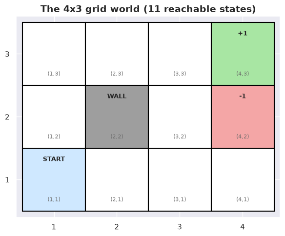

env.states (n=11): [(1, 1), (2, 1), (3, 1), (4, 1), (1, 2), (3, 2), (4, 2), (1, 3), (2, 3), (3, 3), (4, 3)]
env.terminals= {(4, 3): 1.0, (4, 2): -1.0}
env.walls= {(2, 2)}

Key observations:

The environment has 11 reachable states (12 cells minus 1 wall)
Two states are terminal: reaching either ends the episode

Cell 1.2: Stochastic Action Model¶

Goal:

Show why this is an MDP and not a deterministic puzzle
The unreliable actions are the entire source of difficulty

# Create interactive widget showing the stochastic action model.
utils.cell1_2_stochastic_action()

Key observations:

With $\Pr(\text{intended}) = 0.8$ , the agent goes sideways $20\%$ of the time
Walls and boundaries bounce the agent back to its current cell
As p_intended approaches 1.0, the world becomes deterministic
- The intended direction carries probability p_intended
- The two perpendicular directions split the remaining mass equally

Cell 1.3: Transition Model as an Explicit Table¶

Goal:

Make the abstract $\Pr(s' \mid s, a)$ concrete as an actual probability table

# Display the concrete Pr(s' | s, a) table for the START state and Up action.
utils.cell1_3_show_transition_table()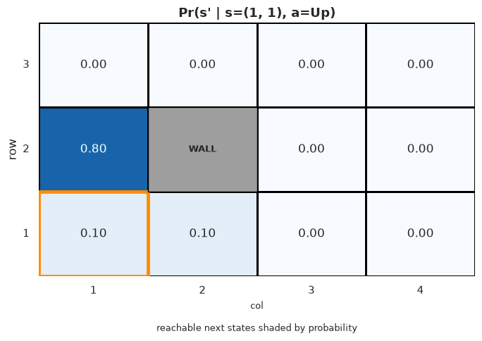

# Show the transition model row for a chosen state and action pair.
utils.cell1_3_transition_table()

Key observations:

The transition model has shape $|S| \times |A| \times |S|$ , but is sparse
- Most next states have zero probability
Each $(s, a)$ row sums to 1.0: it is a probability distribution

# Display the entire transition model for every state-action pair.
utils.cell1_3_full_transition_model()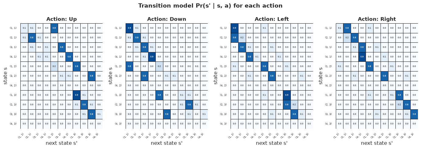


Full transition probability table:

Cell 1.4: Rewards and Episode Returns¶

Goal:

Define the reward structure and connect per-step rewards to discounted return
Show how a single trajectory accumulates $\sum_t \gamma^t R_t$

# Show per-cell rewards and the discounted return of a sample trajectory.
utils.cell1_4_rewards_and_returns()

Key observations:

The small negative living reward -0.04 pushes the agent to finish quickly
- Each non-terminal step costs a little, so wandering is penalized
The discount factor $\gamma$ weights near-term rewards more than distant ones
- Lowering gamma shrinks the contribution of later rewards
Total return depends on the whole sequence of states, not just the final cell
The same path yields different returns as the reward and discount change

Part 2: Solving the MDP with Value Iteration¶

Cell 2.1a: The Bellman Equations for All States¶

Goal:

See the Bellman optimality equation instantiated for every grid cell
Understand how $U(s) = \max_{a \in A(s)} \sum_{s'} \Pr(s' | s, a)[R(s') + \gamma U(s')]$ works out with the actual numbers

The equation for each state shows:

The optimal action (the one that achieves the max)
Each possible next state with its probability, reward, and discounted utility
The resulting utility value, satisfying the Bellman equation

# Pick a state and gamma to see its Bellman optimality equation.
utils.cell2_1_bellman_equations()

Key observations:

The Bellman equation expresses each state’s utility in terms of its possible next states, their rewards, and their discounted utilities
The $\max$ operator selects the best action, making the system nonlinear
Each term shows the exact probability, reward, and discounted utility product that sums to the state’s utility
Higher probabilities weight their corresponding next-state outcomes more heavily in the sum
The optimal action is the one whose expected return is highest
Repeating this update across all states until convergence is value iteration

Cell 2.2: Value Iteration Converging Over Sweeps¶

Goal:

Watch state utilities converge to a fixed point as we sweep the grid
See value information propagate backward from the terminals

# Step through value iteration sweeps and watch utilities converge.
utils.cell2_2_value_iteration()

Key observations:

Utility spreads backward from the terminals
- Cells near the +1 terminal state have high value
- Cells near the -1 terminal state have low value
The change per sweep shrinks geometrically: convergence is guaranteed
- Early sweeps only affect cells adjacent to the terminals
- Later sweeps refine the interior until nothing changes
Higher gamma propagates value further but converges more slowly

Cell 2.1: The Bellman Equation for One State¶

Goal:

Build intuition for the Bellman update on a single state
The full algorithm is just this update applied everywhere

# Show the value of each action at one state under converged utilities.
utils.cell2_1_bellman_one_state()

Key observations

The utility of a state is the value of its best action (not the average)
- Different actions can have very different values at the same state
Each action blends immediate reward with the discounted utility of next states
- The $\max$ operator makes the system nonlinear, so we iterate
- The greedy action is the one whose expected next-state utility is highest
Repeating this max update everywhere is exactly value iteration

Cell 2.3: Extracting the Optimal Policy¶

Goal:

Turn converged utilities into an actionable policy
Take the greedy action in every cell

# Show the greedy policy extracted from converged utilities.
utils.cell2_3_extract_policy()

Key observations:

The policy is derived from utilities, not learned separately
The arrows point toward the action that maximizes expected return
Observed behaviors
- A large negative living reward makes the agent take the short risky path
- A near-zero living reward makes the agent take the long safe path
- Near the -1 terminal the policy steers cautiously when steps are cheap
- Making each step expensive flips the policy toward the shorter risky route

Part 3: Solving the MDP with Policy Iteration¶

Cell 3.1: Policy Evaluation for a Fixed Policy¶

Goal:

Compute the utility of a fixed (possibly bad) policy
This is a simpler linear problem than the full Bellman equation

# When a policy π is fixed (i.e., π(s) specifies a single action for each state),
# the Bellman equation becomes LINEAR because the max operator disappears.
#
# For a fixed policy π:
#   U^π(s) = R(s) + γ ∑_{s'} P(s' | s, π(s)) U^π(s')
#
# This is a system of |S| linear equations in |S| unknowns (the utilities).
# It can be solved directly using linear algebra: (I - γP) U^π = b
#
# In contrast, the optimal Bellman equation has a max over actions:
#   U*(s) = max_a [ R(s) + γ ∑_{s'} P(s' | s, a) U*(s') ]
# which is NONLINEAR and must be solved iteratively (value iteration).
#
# Key insight: Policy evaluation trades the hard nonlinear system for a cheap
# linear one by committing to a fixed action per state first.

# Evaluate a fixed policy by solving the linear Bellman system.
utils.cell3_1_policy_evaluation()

Key observations:

Evaluation is the first half of policy iteration
- Evaluation answers “how good is this policy”, not “what should I do instead”
With a fixed action per state the $\max$ disappears: the equations are linear
- The linear system $(I - \gamma P) U = b$ is solved directly with numpy
A bad policy
- yields low utilities, especially where it steers into -1
- produces visibly low utilities near the -1 terminal

Cell 3.2: Policy Improvement and Iteration to Optimality¶

Goal:

Alternate evaluation and improvement until the policy stops changing
Watch convergence to the optimal policy in a few iterations

https://github.com/gpsaggese/gpsaggese.github.io/blob/maste

https://github.com/gpsaggese/gpsaggese.github.io/tree/gp_scratch/msml610/tutorials/L12_reinforcement_learning/L12_01_gridworld_4x3_utils.py#L1680

# Step through policy iteration rounds and watch arrows flip to optimal.
# Source: https://github.com/gpsaggese/gpsaggese.github.io/blob/main/msml610/tutorials/L12_reinforcement_learning/L12_01_gridworld_4x3_utils.py#L1680
utils.cell3_2_policy_iteration()

Key observations:

Each round evaluates the policy, then makes it greedy with respect to it
- It converges in very few iterations, often fewer than value iteration sweeps
- It terminates exactly when no state changes its action
- Early rounds flip many arrows at once
A stable policy is provably optimal

Cell 3.3: Value Iteration vs Policy Iteration¶

Goal:

Contrast the two exact methods and their convergence behavior
Understand the tradeoff between many cheap sweeps and few expensive rounds

# Compare convergence of value iteration and policy iteration.
utils.cell3_3_compare_solvers()

Key observations:

Value iteration does many cheap sweeps
Policy iteration does few expensive ones
As $\gamma \to 1$ , value iteration needs many more sweeps
Both converge to the same optimal policy
- They are different routes to the same answer

Part 4: Learning Without a Model (Q-Learning)¶

Cell 4.1: Why Reinforcement Learning is Harder Than Planning¶

Goal:

Contrast:
- Planning (knowing the model)
- Learning (discovering through action)
Understand why the same optimal policy takes a harder route in RL
- Same world, blindfolded: the agent no longer has the transition table
- It must learn the value of actions purely from the rewards it stumbles into
- In RL the agent does not know $\Pr(s' \mid s, a)$ or $R(s, a, s')$
- The agent only sees experience tuples $(s, a, r, s')$ as it moves
The goal is unchanged (maximize expected return), but it must learn and act at the same time

Key observations:

Planning evaluates the model
Learning must discover it through action
Every later algorithm in this part sees only $(s, a, r, s')$ tuples
- The same optimal policy is the target, reached by a harder route

Cell 4.2: The Q-Learning Update Rule¶

Goal:

Introduce the single update that powers Q-learning
Show how one experience tuple nudges a Q-value toward a better estimate

# Show how a single experience tuple nudges a Q-value via the TD update.
utils.cell4_2_q_update_rule()

Key observations:

The TD error $r + \gamma \max_{a'} Q(s', a') - Q(s, a)$ measures surprise
The learning rate $\alpha$ controls how aggressively we overwrite the estimate
The update bootstraps from the current estimate of the next state’s value
A larger alpha makes each experience move the estimate further
The TD target combines the observed reward with the discounted next value
With alpha near zero the estimate barely moves; near one it jumps to the target

Cell 4.3: Exploration vs Exploitation with Epsilon-Greedy¶

Goal:

Show why the agent must sometimes act randomly
A purely greedy agent can lock onto a suboptimal path

# Compare state coverage under low vs high exploration.
utils.cell4_3_exploration()

Key observations:

A greedy agent may never visit states off its first decent path
Too much exploration wastes episodes acting randomly
Effective learning needs a balance, often decaying $\epsilon$ over time
Low epsilon concentrates visits on a narrow corridor of states
High epsilon spreads visits broadly but refines actions slowly
The visit heatmap shows exactly which states the agent has explored

Cell 4.4: Watching Q-Learning Learn the Optimal Policy¶

Goal:

Run full Q-learning and watch the learned policy emerge
Compare it to the policy value iteration found with full knowledge

# Train Q-learning and compare its policy to the value iteration optimum.
utils.cell4_4_q_learning_converges()

Key observations:

With enough episodes, Q-learning recovers the same optimal policy
The learning curve is noisy early (exploration) and stabilizes as Q converges
Model-free learning trades sample efficiency for not needing a model
The learned arrows converge to the value iteration policy as episodes grow
Returns rise and flatten as the Q-table stops changing
The same optimal behavior is reached without ever reading the model

Summary: The Mental Model¶

An MDP is defined by states, stochastic actions $\Pr(s' \mid s, a)$ , rewards $R(s, a, s')$ , and a discount $\gamma$
- E.g., the 4x3 grid
When the model is known:
- Value iteration and policy iteration compute the optimal policy exactly by solving the Bellman equations
When the model is unknown
- Q-learning learns the optimal policy from raw experience tuples $(s, a, r, s')$ , balancing exploration and exploitation
All three methods converge to the same optimal policy on the same world: the difference is whether you plan with a model or learn without one