The 4x3 Grid World with Gymnasium - MSML610 -- Tutorials

This notebook mirrors the L12_01_gridworld_4x3 notebook cell-by-cell
Uses a gymnasium.Env subclass for the same 4x3 grid world
The environment exposes P[s][a] (FrozenLake convention) for planning, and step() for model-free learning
The pedagogical arc is identical:
- Build the env -> solve it with full knowledge -> learn without a model
The only difference from the from-scratch version is the API:
- States are integer IDs (0-10) instead of (col, row) tuples
- Actions are integer IDs (0-3) instead of strings
- gymnasium calls reset() and step() instead of direct model access

Gridworld 4x3 Gymnasium¶

Imports¶

%load_ext autoreload
%autoreload 2

import logging

import matplotlib.pyplot as plt
import seaborn as sns

sns.set_style("whitegrid")
plt.rcParams["figure.figsize"] = (14, 5)

The autoreload extension is already loaded. To reload it, use:
  %reload_ext autoreload

import helpers.hnotebook as hnotebook

import L12_02_gridworld_4x3_gymnasium_utils as utils

hnotebook.config_notebook()
_LOG = logging.getLogger(__name__)
utils.init_loggers(_LOG)

WARNING: Logger already initialized: skipping

Part 1: Building the Grid World Environment (Gymnasium)¶

Cell 1.1: The 4x3 Grid and Its States¶

Same layout as the from-scratch version: 4x3 grid with START, +1, -1, WALL
This time, states are gym.spaces.Discrete(11) and actions are gym.spaces.Discrete(4)
The grid world is fully observable (the agent sees its state ID) but stochastic (actions do not always succeed)

# Draw the grid and print the gymnasium observation / action spaces.
utils.cell1_1_show_grid()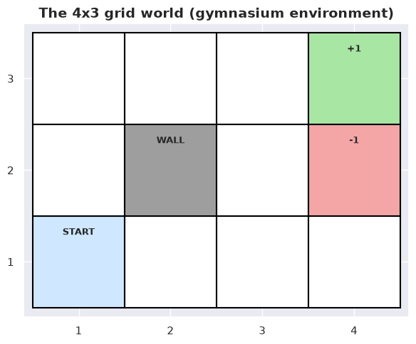

observation_space: Discrete(11)
action_space: Discrete(4)
n_states=11
state id -> cell mapping:
  0 -> (1, 1)
  1 -> (2, 1)
  2 -> (3, 1)
  3 -> (4, 1)
  4 -> (1, 2)
  5 -> (3, 2)
  6 -> (4, 2)
  7 -> (1, 3)
  8 -> (2, 3)
  9 -> (3, 3)
  10 -> (4, 3)
terminal ids: [6, 10]

The environment has 11 reachable states (12 cells minus 1 wall)
Two states are terminal: reaching either ends the episode
State IDs 0-10 map to the same (col, row) cells

Cell 1.2: Stochastic Action Model¶

Goal:

See the stochastic slip model through the gymnasium env.P[s][a] interface
Understand how the intended action and perpendicular slips share probability mass

Grid: Highlighted state with arrow thickness encoding outcome probability Comments: Current parameter values and computed outcome probabilities

# Show how an intended action spreads probability mass through env.P.
utils.cell1_2_stochastic_action()

Cell 1.3: Transition Model from env.P¶

Goal:

See how env.P[s][a] exposes the transition model as (prob, s', reward, terminated) tuples
Understand that planning algorithms read this dict while Q-learning uses step()

Transition heatmap: Probability distribution over next states for the selected (state, action) Transition table: Each outcome with probability, reward, and terminal flag

# Display the explicit transition row from env.P for a chosen (state, action).
utils.cell1_3_transition_table()

Cell 1.4: Rewards and Episode Returns¶

Goal:

Define the reward structure and connect per-step rewards to discounted return
See a sample trajectory rolled out via env.step()

Rewards and trajectory: Per-cell living rewards with a sample path from START Comments: Discounted return computation and step-by-step rewards

# Show per-cell rewards and the discounted return of a sample trajectory.
utils.cell1_4_rewards_and_returns()

Part 2: Solving the MDP with Value Iteration¶

Cell 2.1: The Bellman Equation for One State¶

Goal:

Build intuition for the Bellman update on a single state using integer state and action IDs
See how the Bellman update reads env.P[s][a] to compute Q-values

# Show the value of each action at one state under converged utilities.
utils.cell2_1_bellman_one_state()

Key observations:

The utility of a state is the value of its best action
The max is what makes the system nonlinear, requiring iteration

Cell 2.2: Value Iteration Converging Over Sweeps¶

Goal:

Watch value iteration converge on the gymnasium env.P model
See utility information propagate backward from the terminals

# Step through value iteration sweeps and watch utilities converge.
utils.cell2_2_value_iteration()

Key observations:

Value propagates backward from the terminals, one ring per sweep
The change per sweep shrinks geometrically

Cell 2.3: Extracting the Optimal Policy¶

Goal:

Turn converged utilities into an actionable policy
Take the greedy action in every cell

# Show the greedy policy extracted from converged utilities.
utils.cell2_3_extract_policy()

Key observations:

The living reward controls risk: expensive steps push the agent toward the short risky path; cheap steps let it take the long safe route

Part 3: Solving the MDP with Policy Iteration¶

Cell 3.1: Policy Evaluation for a Fixed Policy¶

Goal:

Compute the utility of a fixed policy by solving $(I - \gamma P) U = b$
Read transition probabilities from env.P[s][a]

# Evaluate a fixed policy by solving the linear Bellman system.
utils.cell3_1_policy_evaluation()

Key observations:

A bad policy yields low utilities, especially near the -1 terminal
Evaluation answers “how good is this policy”

Cell 3.2: Policy Improvement and Iteration to Optimality¶

Goal:

Alternate evaluation and improvement until the policy stops changing
Watch convergence from a deliberately poor policy to the optimal one

# Step through policy iteration rounds and watch arrows flip.
utils.cell3_2_policy_iteration()

Key observations:

Policy iteration typically converges in fewer rounds than value iteration
Each round is more expensive (solving a linear system), but the total wall-clock can still be lower

Cell 3.3: Value Iteration vs Policy Iteration¶

Goal:

Contrast the two exact methods and their convergence behavior
Understand the tradeoff between many cheap sweeps and few expensive rounds

# Compare convergence of the two exact methods.
utils.cell3_3_compare_solvers()

Key observations:

As $\gamma \to 1$ , value iteration needs many more sweeps
Policy iteration is relatively unaffected by gamma

Part 4: Learning Without a Model (Q-Learning)¶

Cell 4.1: Why Reinforcement Learning is Harder Than Planning¶

Goal:

Contrast planning (reading env.P[s][a]) with learning (calling env.step())
Understand why the same optimal policy takes a harder route in RL
The agent calls env.step() and never reads env.P[s][a]
It must learn the value of actions purely from the experience tuples it gets back from each step

# Contrast planning (reads env.P) with learning (calls env.step()).
utils.cell4_1_planning_vs_learning()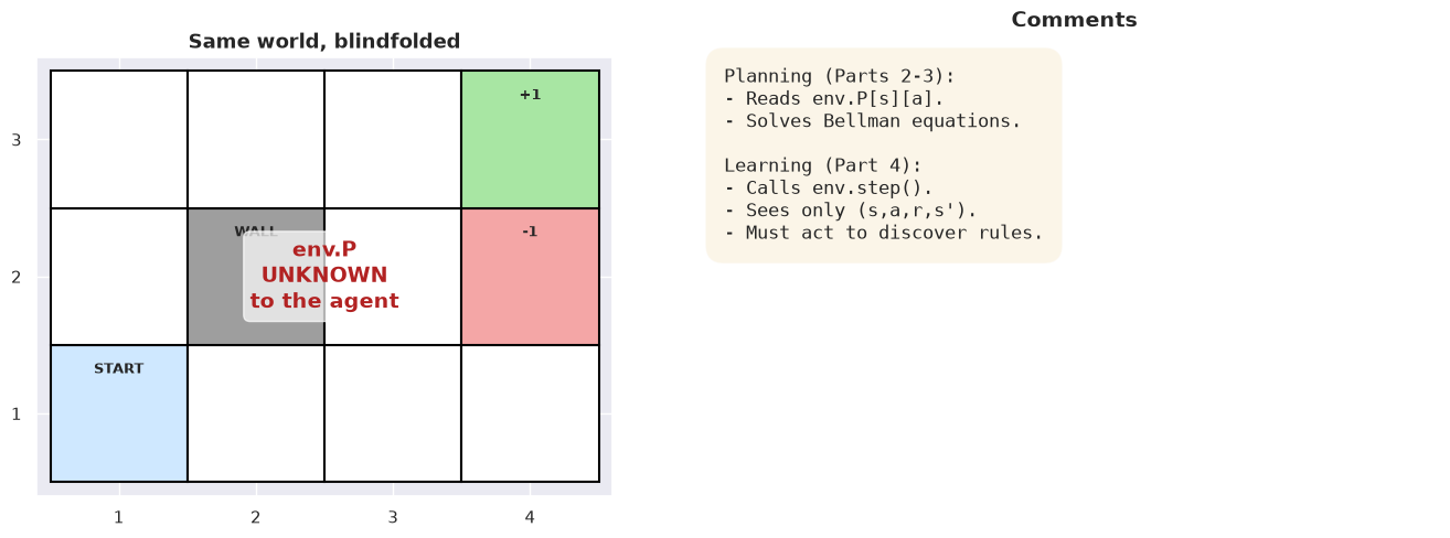

Key observations:

The transition model is hidden behind the gymnasium API
The agent discovers the world by interacting with it

Cell 4.2: The Q-Learning Update Rule¶

Goal:

Introduce the single update that powers Q-learning
Show how one env.step() call produces the TD update tuple

# Show how a single env.step() tuple nudges a Q-value.
utils.cell4_2_q_update_rule()

Key observations:

The TD error measures surprise: the gap between old expectation and observed outcome
No transition probabilities are needed

Cell 4.3: Exploration vs Exploitation with Epsilon-Greedy¶

Goal:

Show why the agent must sometimes act randomly
Compare state coverage at low and high exploration rates

# Compare state coverage under low vs high epsilon using q_learning().
utils.cell4_3_exploration()

Key observations:

The visit heatmap reveals exactly which states the agent has explored
A balance between exploration and exploitation is essential

Cell 4.4: Watching Q-Learning Learn the Optimal Policy¶

Goal:

Run full Q-learning and watch the learned policy emerge
Compare it to the policy value iteration found with full knowledge

# Train Q-learning via env.step() and compare to the planning optimum.
utils.cell4_4_q_learning_converges()

Key observations:

The learned arrows converge to the value iteration arrows as episodes grow
Returns rise and flatten as the Q-table stabilises
This is the payoff: the same optimal behaviour emerges from pure experience, no model required

Summary: The Mental Model¶

A gymnasium.Env subclass is an MDP: its P[s][a] encodes the transition model and its step() lets the agent interact without reading the model
When the model is known (planning), value_iteration() and policy_iteration() read env.P and compute the optimal policy exactly
When the model is unknown (learning), q_learning() calls env.step() and discovers the optimal policy from experience tuples
All three methods converge to the same optimal policy on the same environment -- the difference is whether you plan with the model or learn without it
The gymnasium GridWorldEnv produces exactly the same optimal utilities and policies as the from-scratch GridWorld class