Refuting Causal Estimates - UMD Classes -- Tutorials

This notebook teaches the philosophy and methods of refutation-based validation for causal inference
- Why we cannot prove causality from observational data alone
- How to systematically challenge causal claims using refutation tests
- How to interpret refutation results and decide what to trust
- How to compare competing estimation methods using robustness batteries

Imports¶

%load_ext autoreload
%autoreload 2

# System libraries.
import logging

# Helpers imports.
import helpers.hdbg as hdbg
import helpers.hnotebook as hnotebook

# Notebook-specific utilities.
import dowhy_04_refuting_estimates_utils as darti

_LOG = logging.getLogger(__name__)

# Initialize notebook configuration and logging.
hnotebook.config_notebook()
hdbg.init_logger(verbosity=logging.INFO, use_exec_path=False)
darti.init_loggers(_LOG)

_LOG.info("Notebook initialized")

WARNING: Running in Jupyter
INFO  > cmd='/opt/venv/lib/python3.12/site-packages/ipykernel_launcher.py -f /root/.local/share/jupyter/runtime/kernel-fb9fe491-882f-4da8-8be6-cc7096573778.json'
INFO  Notebook initialized

Cell 1: Why We Cannot Prove Causality¶

Goal: Build intuition about fundamental limitations of causal inference

Key Concepts:

Observational data cannot distinguish between causal and confounded relationships
Many different causal structures produce identical statistical patterns (observational equivalence)
No amount of data can rule out hidden confounders
Karl Popper’s falsification philosophy: we cannot prove causality, but we can try to refute it

Key Insight: Confidence in a causal claim comes from surviving many systematic challenges, not from statistical proof.

# Visualize the fundamental problem: why we cannot prove causality.
darti.cell1_plot_why_we_cannot_prove_causality()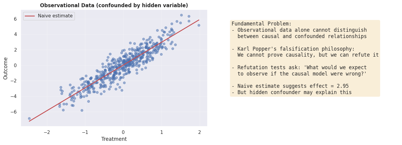

Cell 2: Introduction to Refutation Methods¶

Goal: Survey the landscape of refutation approaches

Two Categories of Refutations:

Negative control refutations: Test necessary conditions that good estimators must satisfy
- Placebo treatment: good estimators find zero effect for fake treatments
- Dummy outcome: estimators should not find spurious effects
- Random confounder: estimates should be stable when adding noise
- Data subsample: effects should be consistent across subsets
Sensitivity analysis: Test robustness when key assumptions are relaxed
- Simulation-based: directly perturb data to simulate confounding
- Partial R² based: use observed variance to bound hidden confounders

Key Principle: If an estimator fails any test (p-value < 0.05), it indicates methodological problems.

# Display a table of refutation methods and interpretation guidance.
darti.cell2_show_refutation_methods_table()


Interpretation guide:
- PASS: Estimator passes the test (result is as expected)
- FAIL: Estimator fails the test (unexpected result at p < 0.05)
- Multiple passes: High confidence in the causal estimate

Cell 3: Simple Synthetic Data with Known Truth¶

Goal: Establish a baseline where we know the true causal effect

Data-Generating Process:

$Z \sim N(0, 1)$ : Hidden confounder
$X = 0.5Z + N(0, 1)$ : Treatment (influenced by confounder)
$Y = 2X + 0.8Z + N(0, 1)$ : Outcome (causal effect = 2)

Challenge: We observe X and Y are correlated, but Z is hidden. Naive estimation will be biased.

# Generate synthetic data with known ground truth.
df, true_ate = darti.cell3_generate_synthetic_data(
    n_samples=500,
    true_ate=2.0,
    confounder_strength=0.8,
    random_state=42,
)

_LOG.info(f"Generated {len(df)} samples with true ATE = {true_ate}")

INFO  Generated 500 samples with true ATE = 2.0

# Visualize the data-generating process.
darti.cell3_visualize_data(df, true_ate)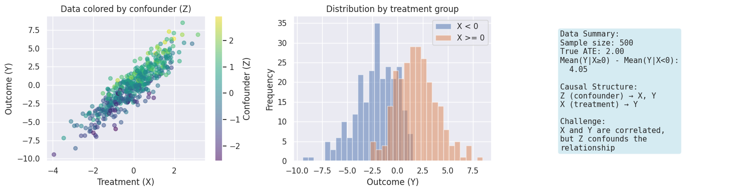

Cell 4: Naive Estimation Reveals the Problem¶

Goal: Demonstrate that naive methods can give very wrong answers

What We’ll Do:

Estimate the treatment effect using naive linear regression (ignoring Z)
Compare to ground truth to quantify bias
Discuss why this happens: omitted variable bias

# Estimate causal effect using naive methods.
naive_results = darti.cell4_naive_estimation(df, true_ate)

_LOG.info(f"Naive estimate: {naive_results['estimate']:.3f}")
_LOG.info(f"True ATE: {naive_results['true_ate']:.3f}")
_LOG.info(f"Bias: {naive_results['bias']:.3f}")

INFO  Naive estimate: 2.277
INFO  True ATE: 2.000
INFO  Bias: 0.277

# Visualize the bias in naive estimation.
darti.cell4_visualize_bias(naive_results)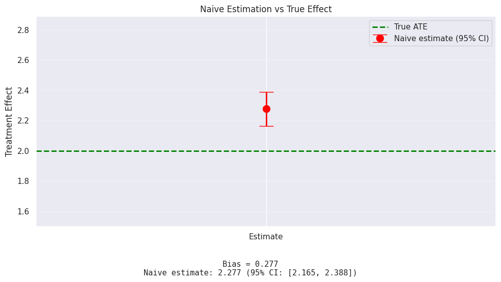

Cell 5: Placebo Treatment Refutation¶

Goal: Learn how placebo treatment tests detect spurious effects

Concept: If we assign a fake treatment that cannot possibly have a causal effect, a good estimator should find zero effect. A bad estimator finds spurious effects.

Interpretation:

Pass: Placebo effects distributed around zero, p-value > 0.05
Fail: Placebo effects systematically non-zero, p-value < 0.05

# Run placebo treatment refutation.
placebo_results = darti.cell5_run_placebo_refutation(
    df,
    true_ate,
    n_placebos=50,
    random_state=42,
)

# Visualize the distribution of placebo effects.
darti.cell5_visualize_placebo(placebo_results)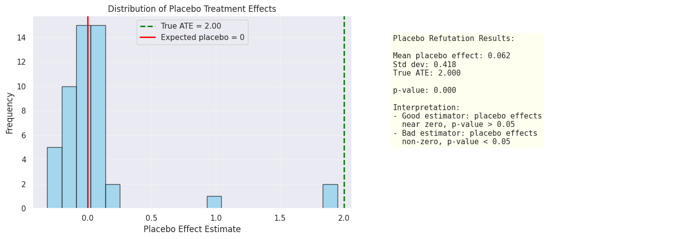

Cell 6: Dummy Outcome Refutation¶

Goal: Learn how dummy outcome tests reveal systematic bias

Concept: Create artificial outcome variables with no causal relationship to treatment. A good estimator should find zero effect on all dummy outcomes.

Interpretation:

Pass: True effect is extreme in the dummy distribution (good signal)
Fail: True effect in the center of dummy distribution (spurious)

# Run dummy outcome refutation.
dummy_results = darti.cell6_run_dummy_outcome_refutation(
    df,
    true_ate,
    n_dummy=100,
    random_state=42,
)

# Visualize the distribution of dummy outcome effects.
darti.cell6_visualize_dummy_outcome(dummy_results)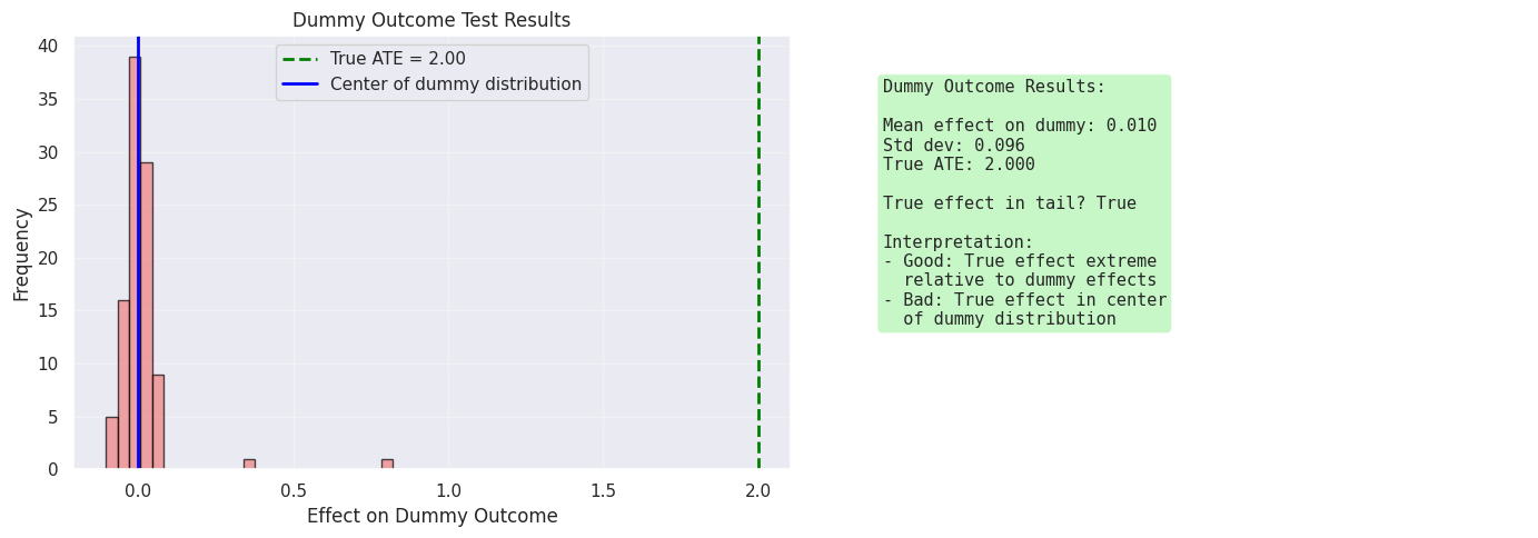

Cell 7: Random Common Cause Refutation¶

Goal: Test whether estimator incorrectly adjusts for irrelevant confounders

Concept: Introduce random variables as fake confounders. A good estimator should not change estimates when we wrongly adjust for them.

Interpretation:

Pass: Estimates stable despite random confounders (low std dev)
Fail: Estimates vary widely with confounder choice (high std dev)

# Run random confounder refutation.
confounder_results = darti.cell7_run_random_confounder_refutation(
    df,
    n_confounders=10,
    random_state=42,
)

# Visualize sensitivity to random confounders.
darti.cell7_visualize_random_confounder(confounder_results)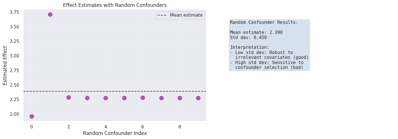

Cell 8: Data Subsample Refutation¶

Goal: Test consistency and stability of estimates across data subsets

Concept: If the causal relationship is real and estimation is robust, the effect estimate should be consistent across random subsamples.

Interpretation:

Pass: Subsample estimates concentrated with low variance (stable)
Fail: Subsample estimates highly variable (unstable)

# Run subsample refutation.
subsample_results = darti.cell8_run_subsample_refutation(
    df,
    subsample_fraction=0.8,
    n_subsamples=50,
    random_state=42,
)

# Visualize consistency across subsamples.
darti.cell8_visualize_subsample(subsample_results)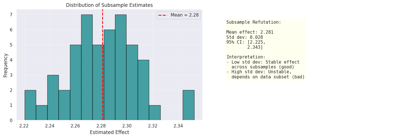

Cell 9: Sensitivity Analysis to Unobserved Confounding¶

Goal: Understand robustness when key assumptions are violated

Core Concept: We cannot observe hidden confounders, but we can test robustness by assuming they exist and checking if conclusions hold.

Three Approaches:

Simulation-based: directly add noise to simulate confounding
Partial R² based: use observed variance to bound hidden confounder strength
Reisz estimator based: derive bounds under unobserved confounding violations

Key Question: At what level of hidden confounding would conclusions reverse?

# Run sensitivity analysis.
sensitivity_results = darti.cell9_sensitivity_analysis(
    df,
    confounder_strengths=[0, 0.25, 0.5, 0.75, 1.0, 1.5, 2.0],
    random_state=42,
)

# Visualize sensitivity bounds.
darti.cell9_visualize_sensitivity(sensitivity_results)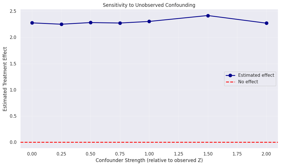

Cell 10: Comparing Multiple Estimators via Refutations¶

Goal: Use refutation tests to rank competing causal estimation methods

Approach:

Apply all refutation methods to multiple estimators
For each estimator, collect results from previous cells
Create comparison scorecard: which estimators pass most tests?

Interpretation:

Estimator passing all tests: most trustworthy
Estimator failing tests: methodological issues

# Compare multiple estimation methods.
comparison_results = darti.cell10_compare_estimators(df)

# Visualize comparison of estimators.
darti.cell10_visualize_comparison(comparison_results)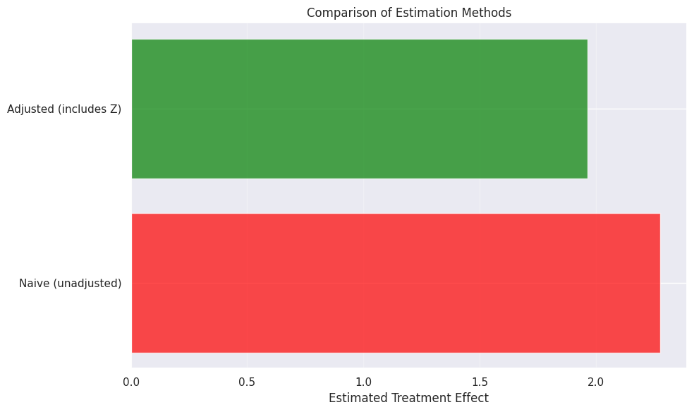

Cell 11: Real Data Example: Job Training Impact¶

Goal: Apply complete refutation workflow to realistic problem with stakes

Scenario: Evaluate impact of job training program on earnings

Data: Individuals with varying training participation and post-training earnings, with potential selection bias from unmeasured motivation.

Question: Does the training program actually increase earnings, or is the observed effect due to selection bias?

# Create realistic job training dataset.
job_df = darti.cell11_create_job_training_data(
    n_samples=1000,
    random_state=42,
)

_LOG.info(f"Generated job training dataset with {len(job_df)} individuals")
job_df.head()

---------------------------------------------------------------------------
ValueError                                Traceback (most recent call last)
Cell In[21], line 2
      1 # Create realistic job training dataset.
----> 2 job_df = darti.cell11_create_job_training_data(
      3     n_samples=1000,
      4     random_state=42,
      5 )

File /git_root/tutorials/dowhy/dowhy_04_refuting_estimates_utils.py:817, in cell11_create_job_training_data(n_samples, random_state)
    812 motivation = (education + age / 10) / 3 + rng.normal(0, 0.3, n_samples)
    813 training = (motivation > np.median(motivation)).astype(int)
    814 post_income = (
    815     40000
    816     + 1.5 * education * 1000
--> 817     + (2000 if training else 0)
    818     + motivation * 5000
    819     + rng.normal(0, 5000, n_samples)
    820 )
    821 df = pd.DataFrame({
    822     "Age": age,
    823     "Education": education,
   (...)    827     "Post_Income": post_income,
    828 })
    829 return df

ValueError: The truth value of an array with more than one element is ambiguous. Use a.any() or a.all()

# Analyze training impact using naive and adjusted estimators.
darti.cell11_analyze_job_training(job_df)

Cell 12: Synthesis and Decision Framework¶

Goal: Develop practical judgment about when to trust causal estimates

Key Takeaway: Causal inference is about finding robust signals that survive systematic challenges, not about achieving statistical proof.

Decision Framework:

Run all applicable refutation tests
Compare results across tests
Decide: are conclusions robust or fragile?
Communicate findings honestly, including limitations

# Display practical checklist for refutation analysis.
darti.cell12_refutation_checklist()