PGMPy Probabilistic Inference API
A guided exploration of pgmpy’s core probabilistic inference abstractions:
- Building Bayesian networks
- Inference engines (VariableElimination, BeliefPropagation)
- Query methods (observational inference, MAP queries)
- Evidence-based conditioning
Imports and Setup
%load_ext autoreload
%autoreload 2

import logging
import sys
import warnings

warnings.filterwarnings('ignore')
from pgmpy.models import DiscreteBayesianNetwork
from pgmpy.factors.discrete import TabularCPD
from pgmpy.inference import VariableElimination, BeliefPropagation
from pgmpy.estimators import MaximumLikelihoodEstimator
import pandas as pd
import numpy as np# # To install additional packages, use:
# import helpers.hmodule as hmodule
# hmodule.install_module_if_not_present(
# ["pygraphviz"],
# use_activate=True,
# use_sudo=False,
# venv_path="/opt/venv",
# )# Use this for most notebooks.
import helpers.htutorial as htutori
htutori.config_notebook()
# Import pgmpy utilities.
import tutorials.pgmpy.pgmpy_utils as tpgpguti
# Initialize logger.
logging.basicConfig(level=logging.INFO)
_LOG = logging.getLogger(__name__)
#utils.init_loggers(_LOG)
# Convert `display` into `print()` when running outside IPython.
try:
from IPython.display import display
except ImportError:
display = print # type: ignorePart 1: Library Overview
What Problem Does PGMPy Solve?
PGMPy enables probabilistic reasoning over graphical models:
- Graphical Models: Represent complex probability distributions as graphs where nodes are variables and edges encode dependencies
- Bayesian Networks: Directed acyclic graphs (DAGs) representing causal and statistical relationships
- Probabilistic Inference: Answer probability questions given observed evidence: “What is P(X=x | Y=y)?”
- MAP Queries: Find most probable variable assignments given evidence
Key Abstractions
- BayesianNetwork: The graph structure (nodes and edges)
- TabularCPD: Conditional probability distributions (quantify relationships)
- InferenceEngine (VariableElimination, BeliefPropagation): Compute probabilities given evidence
- Query Results: Distributions over variables conditioned on evidence
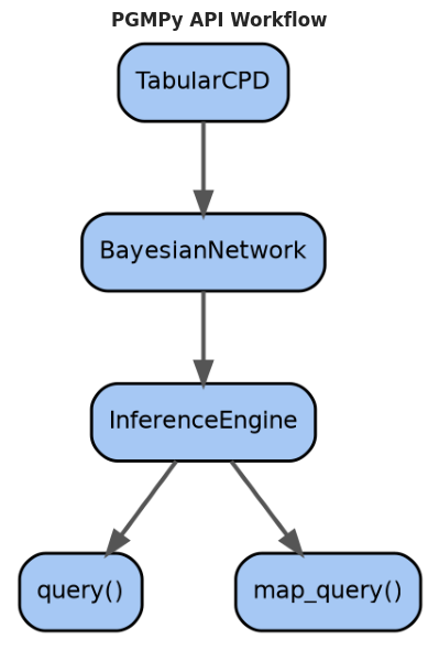
How the Pieces Fit Together
import networkx as nx
import helpers.hgraphviz as hgraphv

# Create a directed graph showing the API workflow.
G = nx.DiGraph()
G.add_edges_from([
    ('BayesianNetwork', 'InferenceEngine'),
    ('TabularCPD', 'BayesianNetwork'),
    ('InferenceEngine', 'query()'),
    ('InferenceEngine', 'map_query()'),
])

# Visualize using graphviz.
_ = hgraphv.plot_causal_dag(
    G,
    title='PGMPy API Workflow',
    figsize=(8, 6)
)
Part 2: Core Primitives
Primitive 1: DiscreteBayesianNetwork
Represents the graph structure (directed acyclic graph).
Mental Model
A BayesianNetwork is:
- A directed acyclic graph (DAG) encoding independence assumptions
- An edge A → B means “A probabilistically influences B”
- Each node requires a Conditional Probability Distribution (CPD)
- Nodes without parents are root nodes (prior distributions)
- Nodes with parents are conditional on those parents
Minimal Construction
# Smallest possible Bayesian network: 2 nodes with 1 edge.
model = DiscreteBayesianNetwork([('A', 'B')])

print(f"Type: {type(model)}")
print(f"Nodes: {model.nodes()}")
print(f"Edges: {model.edges()}")
Type: <class 'pgmpy.models.DiscreteBayesianNetwork.DiscreteBayesianNetwork'>
Nodes: ['A', 'B']
Edges: [('A', 'B')]
Inspect the Object
# View important attributes.
print(f"Has CPDs: {model.get_cpds()}")

# DiscreteBayesianNetwork is invalid without CPDs.
try:
    result = model.check_model()
    print(f"Check valid: {result}")
    print("Model is valid")
except Exception as e:
    print(f"Model is INVALID: {type(e).__name__}")
    print(f"  Reason: Missing CPDs for nodes {model.nodes()}")
Has CPDs: []
Model is INVALID: ValueError
Reason: Missing CPDs for nodes ['A', 'B']
Important Methods
# Exploring the network structure.
model = DiscreteBayesianNetwork([('A', 'B'), ('A', 'C'), ('B', 'C')])

print(f"Parents of B: {model.get_parents('B')}")
print(f"Children of A: {model.get_children('A')}")
print(f"All ancestors of C: {model.get_ancestors('C')}")
Parents of B: ['A']
Children of A: ['B', 'C']
All ancestors of C: {'A', 'B', 'C'}
Primitive 2: TabularCPD (Conditional Probability Distribution)
Quantifies the relationship between variables as a probability table.
Mental Model
A TabularCPD is:
- A probability table quantifying relationships between variables
- For a node with no parents: a prior probability distribution (column vector)
- For a node with parents: conditional distributions (one column per parent configuration)
- Specifies P(Variable=value | ParentA=val_a, ParentB=val_b, ...)
- Each column sums to 1.0 (valid probability distribution)
- Essential for converting the graph structure into concrete probabilities
CPD with No Parents
# CPD for a node with no parents (prior).
cpd_a = TabularCPD(
    variable='A',
    # A can take 2 values: 0 or 1.
    # `card` stands for cardinality.
    variable_card=2,
    # P(A=0)=0.6, P(A=1)=0.4.
    values=[[0.6], [0.4]]
)

print(f"Type: {type(cpd_a)}")
print(cpd_a)
Type: <class 'pgmpy.factors.discrete.CPD.TabularCPD'>
+------+-----+
| A(0) | 0.6 |
+------+-----+
| A(1) | 0.4 |
+------+-----+
CPD with Parents
# CPD for B given A (B has parent A).
# B's distribution depends on A's value.
# P(B=0 | A=0)=0.9, P(B=0 | A=1)=0.2.
# P(B=1 | A=0)=0.1, P(B=1 | A=1)=0.8.
cpd_b = TabularCPD(
    variable='B',
    variable_card=2,
    values=[
        [0.9, 0.2],
        [0.1, 0.8]
    ],
    evidence=['A'],
    evidence_card=[2]
)

print(cpd_b)
+------+------+------+
| A | A(0) | A(1) |
+------+------+------+
| B(0) | 0.9 | 0.2 |
+------+------+------+
| B(1) | 0.1 | 0.8 |
+------+------+------+
The CPD table shows the conditional probability distribution of B given A:
- Each column represents one value of the parent variable A
- Column A(0): P(B=0 | A=0)=0.9, P(B=1 | A=0)=0.1
- Column A(1): P(B=0 | A=1)=0.2, P(B=1 | A=1)=0.8
- Each column sums to 1.0 (valid probability distribution)
factor_to_dataframe(cpd_b)Loading...
Important Methods
# Inspect a CPD.
print(f"Variable: {cpd_b.variable}")
print(f"Cardinality (num values): {cpd_b.cardinality}")
print(f"Evidence: {cpd_b.variables[1:]}")
print(f"Evidence cardinality: {cpd_b.cardinality[1:]}")

# Access probability values.
print(f"\nP(B=0 | A=1): {cpd_b.values[0, 1]}")
print(f"P(B=1 | A=0): {cpd_b.values[1, 0]}")
Variable: B
Cardinality (num values): [2 2]
Evidence: ['A']
Evidence cardinality: [2]
P(B=0 | A=1): 0.2
P(B=1 | A=0): 0.1
Primitive 3: InferenceEngine (VariableElimination)
Computes posterior probabilities given evidence.
Mental Model
An InferenceEngine is:
- An algorithm that computes posterior probabilities from a graphical model
- Takes a fitted BayesianNetwork (with CPDs)
- Answers conditional probability questions: P(query_vars | evidence)
- Different implementations
VariableElimination: Exact, efficient for many practical modelsBeliefPropagation: Exact, optimized for repeated queries
Minimal Construction and Setup
# Create a complete model.
model = DiscreteBayesianNetwork([('A', 'B')])

# Add CPDs.
cpd_a = TabularCPD('A', 2, [[0.6], [0.4]])
cpd_b = TabularCPD(
    'B', 2,
    [[0.9, 0.2], [0.1, 0.8]],
    evidence=['A'], evidence_card=[2]
)

model.add_cpds(cpd_a, cpd_b)
model.check_model()

# Create inference engine: computes posterior probabilities given evidence.
inference = VariableElimination(model)

print(f"Type: {type(inference)}")
print(f"Model: {inference.model.nodes()}")
Type: <class 'pgmpy.inference.ExactInference.VariableElimination'>
Model: ['A', 'B']
# Import helper functions from pgmpy_utils.
draw_pgmpy_model = tpgpguti.draw_pgmpy_model
_ = draw_pgmpy_model(model)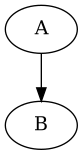
Important Methods
# Query: compute P(B | A=1).
result = inference.query(variables=['B'], evidence={'A': 1})

print(f"Type of result: {type(result)}")
print(result)
print(f"\nP(B=0 | A=1) = {result.values[0]}")
print(f"P(B=1 | A=1) = {result.values[1]}")
Type of result: <class 'pgmpy.factors.discrete.DiscreteFactor.DiscreteFactor'>
+------+----------+
| B | phi(B) |
+======+==========+
| B(0) | 0.2000 |
+------+----------+
| B(1) | 0.8000 |
+------+----------+
P(B=0 | A=1) = 0.2
P(B=1 | A=1) = 0.8
# Import helper functions from pgmpy_utils.
factor_to_dataframe = tpgpguti.factor_to_dataframefactor_to_dataframe(result)Loading...
Primitive 4: Query Results
The output of inference queries: probability distributions.
# Query result is a Factor object.
result = inference.query(variables=['B'], evidence={'A': 0})

print(f"Type: {type(result)}")
print(f"Variables: {result.variables}")
print(f"Cardinality: {result.cardinality}")
print(f"\nAs array: {result.values}")
Type: <class 'pgmpy.factors.discrete.DiscreteFactor.DiscreteFactor'>
Variables: ['B']
Cardinality: [2]
As array: [0.9 0.1]
Part 3: Composition Examples
Example 1: Minimal End-to-End Workflow
Rain → Sprinkler → Grass Wet
# 1. Define structure.
model = DiscreteBayesianNetwork([('Rain', 'GrassWet'), ('Sprinkler', 'GrassWet')])

# 2. Define CPDs.
cpd_rain = TabularCPD('Rain', 2, [[0.8], [0.2]])  # Usually no rain.
cpd_sprinkler = TabularCPD('Sprinkler', 2, [[0.6], [0.4]])  # Usually off.

# 3. Grass wet depends on both Rain and Sprinkler.
cpd_grass = TabularCPD(
    'GrassWet', 2,
    [
        [0.99, 0.1, 0.1, 0.01],  # P(Grass=dry | ...).
        [0.01, 0.9, 0.9, 0.99]   # P(Grass=wet | ...).
    ],
    evidence=['Rain', 'Sprinkler'],
    evidence_card=[2, 2]
)

model.add_cpds(cpd_rain, cpd_sprinkler, cpd_grass)
model.check_model()

print("Model is valid!")
print(f"Nodes: {model.nodes()}")
print(f"Edges: {model.edges()}")
Model is valid!
Nodes: ['Rain', 'GrassWet', 'Sprinkler']
Edges: [('Rain', 'GrassWet'), ('Sprinkler', 'GrassWet')]
_ = draw_pgmpy_model(model)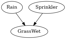
# 4. Create inference engine and query.
inference = VariableElimination(model)

# Query 1: Grass is wet, what's probability of rain?
result = inference.query(variables=['Rain'], evidence={'GrassWet': 1})
print("P(Rain | Grass=wet):")
print(result)

# Query 2: Both rain and sprinkler, what's probability grass is wet?
result = inference.query(
    variables=['GrassWet'],
    evidence={'Rain': 1, 'Sprinkler': 1}
)
print("\nP(Grass | Rain=yes, Sprinkler=yes):")
print(result)
P(Rain | Grass=wet):
+---------+-------------+
| Rain | phi(Rain) |
+=========+=============+
| Rain(0) | 0.6100 |
+---------+-------------+
| Rain(1) | 0.3900 |
+---------+-------------+
P(Grass | Rain=yes, Sprinkler=yes):
+-------------+-----------------+
| GrassWet | phi(GrassWet) |
+=============+=================+
| GrassWet(0) | 0.0100 |
+-------------+-----------------+
| GrassWet(1) | 0.9900 |
+-------------+-----------------+
Example 2: Add Multi-State Variables
Temperature (cold, warm, hot) → Comfort (bad, good)
# Variables can have more than 2 states.
model = DiscreteBayesianNetwork([('Temperature', 'Comfort')])

# Temperature: 0=cold, 1=warm, 2=hot.
cpd_temp = TabularCPD(
    'Temperature', 3,
    [[0.3], [0.5], [0.2]]  # 30% cold, 50% warm, 20% hot.
)

# Comfort: 0=bad, 1=good.
# Changes based on temperature.
cpd_comfort = TabularCPD(
    'Comfort', 2,
    [
        [0.8, 0.1, 0.6],  # P(Comfort=bad | ...).
        [0.2, 0.9, 0.4]   # P(Comfort=good | ...).
    ],
    evidence=['Temperature'],
    evidence_card=[3]
)

model.add_cpds(cpd_temp, cpd_comfort)
model.check_model()

inference = VariableElimination(model)
result = inference.query(variables=['Temperature'], evidence={'Comfort': 1})

print("P(Temperature | Comfort=good):")
for i, val in enumerate(result.values):
    print(f"  P(Temp={i}) = {val:.3f}")
P(Temperature | Comfort=good):
P(Temp=0) = 0.102
P(Temp=1) = 0.763
P(Temp=2) = 0.136
_ = draw_pgmpy_model(model)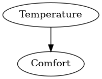
Example 3: Chain Structure
X → Y → Z (three-node chain)
model = DiscreteBayesianNetwork([('X', 'Y'), ('Y', 'Z')])

cpd_x = TabularCPD('X', 2, [[0.4], [0.6]])
cpd_y = TabularCPD(
    'Y', 2,
    [[0.9, 0.3], [0.1, 0.7]],
    evidence=['X'], evidence_card=[2]
)
cpd_z = TabularCPD(
    'Z', 2,
    [[0.8, 0.2], [0.2, 0.8]],
    evidence=['Y'], evidence_card=[2]
)

model.add_cpds(cpd_x, cpd_y, cpd_z)
model.check_model()True_ = draw_pgmpy_model(model)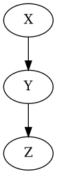
inference = VariableElimination(model)

# Query with evidence at the beginning.
result = inference.query(variables=['Z'], evidence={'X': 1})
print("P(Z | X=1):")
print(result)

# Query with evidence in the middle.
result = inference.query(variables=['X'], evidence={'Z': 1})
print("\nP(X | Z=1) [backwards inference]:")
print(result)
P(Z | X=1):
+------+----------+
| Z | phi(Z) |
+======+==========+
| Z(0) | 0.3800 |
+------+----------+
| Z(1) | 0.6200 |
+------+----------+
P(X | Z=1) [backwards inference]:
+------+----------+
| X | phi(X) |
+======+==========+
| X(0) | 0.2185 |
+------+----------+
| X(1) | 0.7815 |
+------+----------+
Example 4: V-Structure (Collider)
A ← B → C (classic collider pattern)
# V-structure: both A and C point to B.
model = DiscreteBayesianNetwork([('A', 'B'), ('C', 'B')])

cpd_a = TabularCPD('A', 2, [[0.5], [0.5]])
cpd_c = TabularCPD('C', 2, [[0.5], [0.5]])

# B depends on both A and C.
cpd_b = TabularCPD(
    'B', 2,
    [
        [0.99, 0.6, 0.6, 0.05],  # P(B=0 | ...).
        [0.01, 0.4, 0.4, 0.95]   # P(B=1 | ...).
    ],
    evidence=['A', 'C'],
    evidence_card=[2, 2]
)

model.add_cpds(cpd_a, cpd_c, cpd_b)
model.check_model()True_ = draw_pgmpy_model(model)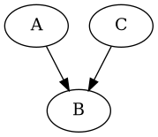
inference = VariableElimination(model)

# Without evidence on B, A and C are independent.
# With evidence on B, they become dependent (explaining away).
result_before = inference.query(variables=['A'], evidence={'C': 1})
result_after = inference.query(variables=['A'], evidence={'B': 1, 'C': 1})

print("P(A | C=1) [without B]:")
print(result_before.values)
print("\nP(A | C=1, B=1) [with B]:")
print(result_after.values)
print("\nNote: Probabilities change when B is observed (explaining away effect)")
P(A | C=1) [without B]:
[0.5 0.5]
P(A | C=1, B=1) [with B]:
[0.2962963 0.7037037]
Note: Probabilities change when B is observed (explaining away effect)
Part 4: API Patterns
Pattern 1: Model Construction and Validation
# Pattern: define structure > add CPDs > validate > create engine.

# Step 1: Structure.
model = DiscreteBayesianNetwork([('A', 'B'), ('B', 'C')])

# Step 2: Add CPDs.
cpd_a = TabularCPD('A', 2, [[0.3], [0.7]])
cpd_b = TabularCPD(
    'B', 2,
    [[0.8, 0.2], [0.2, 0.8]],
    evidence=['A'], evidence_card=[2]
)
cpd_c = TabularCPD(
    'C', 2,
    [[0.9, 0.1], [0.1, 0.9]],
    evidence=['B'], evidence_card=[2]
)
model.add_cpds(cpd_a, cpd_b, cpd_c)

# Step 3: Validation.
is_valid = model.check_model()
print(f"Model valid: {is_valid}")

# Step 4: Create inference engine.
inference = VariableElimination(model)
Model valid: True
Pattern 2: Query Pattern
Basic query: inference.query(variables, evidence)
# Pattern: query(variables=[...], evidence={...}).
# Returns posterior distribution P(variables | evidence).

# Single variable, no evidence.
result = inference.query(variables=['A'])
print("P(A): prior distribution")
print(result)

# Single variable with evidence.
result = inference.query(variables=['C'], evidence={'A': 1})
print("\nP(C | A=1): posterior distribution")
print(result)

# Multiple variables with evidence.
result = inference.query(variables=['A', 'B'], evidence={'C': 0})
print("\nP(A, B | C=0): joint posterior")
print(result)
P(A): prior distribution
+------+----------+
| A | phi(A) |
+======+==========+
| A(0) | 0.3000 |
+------+----------+
| A(1) | 0.7000 |
+------+----------+
P(C | A=1): posterior distribution
+------+----------+
| C | phi(C) |
+======+==========+
| C(0) | 0.2600 |
+------+----------+
| C(1) | 0.7400 |
+------+----------+
P(A, B | C=0): joint posterior
+------+------+------------+
| A | B | phi(A,B) |
+======+======+============+
| A(0) | B(0) | 0.5347 |
+------+------+------------+
| A(0) | B(1) | 0.0149 |
+------+------+------------+
| A(1) | B(0) | 0.3119 |
+------+------+------------+
| A(1) | B(1) | 0.1386 |
+------+------+------------+
Pattern 3: MAP Query Pattern
Find the most probable assignment.
# Pattern: map_query(variables, evidence).
# Returns most probable variable assignment given evidence.

# Most probable value of C given A=1.
result = inference.map_query(variables=['C'], evidence={'A': 1})
print(f"MAP(C | A=1): {result}")
print(f"Interpretation: Most likely value of C is {result['C']}")
Loading...
Loading...
MAP(C | A=1): {'C': 1}
Interpretation: Most likely value of C is 1
# Most probable joint assignment.
result = inference.map_query(variables=['B', 'C'], evidence={'A': 0})
print(f"\nMAP(B, C | A=0): {result}")
print(f"Interpretation: Most likely (B, C) = ({result['B']}, {result['C']})")
Loading...
Loading...
MAP(B, C | A=0): {'B': 0, 'C': 0}
Interpretation: Most likely (B, C) = (0, 0)
Pattern 4: Inference Engine Alternatives
# VariableElimination: Default, efficient for many models.
inference_ve = VariableElimination(model)
result_ve = inference_ve.query(variables=['C'], evidence={'A': 1})

# BeliefPropagation: Optimized for repeated queries.
# Note: Works best on singly-connected networks.
try:
    inference_bp = BeliefPropagation(model)
    result_bp = inference_bp.query(variables=['C'], evidence={'A': 1})
    print("Both engines produce the same result:")
    print(f"VariableElimination: {result_ve.values}")
    print(f"BeliefPropagation:   {result_bp.values}")
except Exception as e:
    print(f"BeliefPropagation note: {e}")
Both engines produce the same result:
VariableElimination: [0.26 0.74]
BeliefPropagation: [0.26 0.74]
Pattern 5: Evidence Specification
# Evidence is specified as {variable: value}.
# Can use multiple pieces of evidence.

# Single observation.
result = inference.query(variables=['A'], evidence={'C': 1})
print("P(A | C=1)")

# Multiple observations.
result = inference.query(
    variables=['A'],
    evidence={'B': 1, 'C': 0}
)
print("\nP(A | B=1, C=0)")
print(result)

# Querying variables can also have evidence.
result = inference.query(
    variables=['A', 'B'],
    evidence={'C': 1}
)
print("\nP(A, B | C=1) - joint distribution of A and B.")
print(result)
P(A | C=1)
P(A | B=1, C=0)
+------+----------+
| A | phi(A) |
+======+==========+
| A(0) | 0.0968 |
+------+----------+
| A(1) | 0.9032 |
+------+----------+
P(A, B | C=1) - joint distribution of A and B.
+------+------+------------+
| A | B | phi(A,B) |
+======+======+============+
| A(0) | B(0) | 0.0403 |
+------+------+------------+
| A(0) | B(1) | 0.0906 |
+------+------+------------+
| A(1) | B(0) | 0.0235 |
+------+------+------------+
| A(1) | B(1) | 0.8456 |
+------+------+------------+
Part 6: Interactive Exploration
Experiment 1: How Does Evidence Change Posteriors?
# Simple model: Cause > Effect.
model = DiscreteBayesianNetwork([('Cause', 'Effect')])
cpd_cause = TabularCPD('Cause', 2, [[0.5], [0.5]])  # Cause is equally likely.
cpd_effect = TabularCPD(
    'Effect', 2,
    [[0.95, 0.1], [0.05, 0.9]],  # Effect strongly correlated with Cause.
    evidence=['Cause'], evidence_card=[2]
)
model.add_cpds(cpd_cause, cpd_effect)
model.check_model()

inference = VariableElimination(model)

# Prior on Cause (no evidence).
prior = inference.query(variables=['Cause'])
print("Prior P(Cause):")
print(f"  P(Cause=0) = {prior.values[0]:.3f}")
print(f"  P(Cause=1) = {prior.values[1]:.3f}")

# Posterior given Effect=1 (strong evidence for Cause).
posterior = inference.query(variables=['Cause'], evidence={'Effect': 1})
print("\nPosterior P(Cause | Effect=1):")
print(f"  P(Cause=0) = {posterior.values[0]:.3f}")
print(f"  P(Cause=1) = {posterior.values[1]:.3f}")

print("\nObservation: Effect=1 makes Cause=1 much more likely!")
print(f"Belief shift: {prior.values[1]:.3f} → {posterior.values[1]:.3f}")
Prior P(Cause):
P(Cause=0) = 0.500
P(Cause=1) = 0.500
Posterior P(Cause | Effect=1):
P(Cause=0) = 0.053
P(Cause=1) = 0.947
Observation: Effect=1 makes Cause=1 much more likely!
Belief shift: 0.500 → 0.947
Experiment 2: Why Variable Cardinality Matters
# Create two models: one with 2 states, one with 5 states.

# Binary model.
model_binary = DiscreteBayesianNetwork([('Weather', 'Traffic')])
cpd_w = TabularCPD('Weather', 2, [[0.7], [0.3]])
cpd_t = TabularCPD(
    'Traffic', 2,
    [[0.95, 0.3], [0.05, 0.7]],
    evidence=['Weather'], evidence_card=[2]
)
model_binary.add_cpds(cpd_w, cpd_t)
model_binary.check_model()

inf_binary = VariableElimination(model_binary)
result = inf_binary.query(variables=['Weather'], evidence={'Traffic': 1})
print("Binary model (Weather: clear/rainy):")
print(f"  CPD table size: 2x2")
print(result)

# Multi-state model.
model_multi = DiscreteBayesianNetwork([('Weather', 'Traffic')])
cpd_w = TabularCPD('Weather', 5, [[0.5], [0.2], [0.15], [0.1], [0.05]])
cpd_t = TabularCPD(
    'Traffic', 3,
    [
        [0.9, 0.4, 0.2, 0.1, 0.05],  # P(T=light)
        [0.08, 0.5, 0.5, 0.4, 0.3],  # P(T=moderate)
        [0.02, 0.1, 0.3, 0.5, 0.65]  # P(T=heavy)
    ],
    evidence=['Weather'], evidence_card=[5]
)
model_multi.add_cpds(cpd_w, cpd_t)
model_multi.check_model()

inf_multi = VariableElimination(model_multi)
result = inf_multi.query(variables=['Weather'], evidence={'Traffic': 2})
print("\nMulti-state model (Weather: 5 states, Traffic: 3 states):")
print(f"  CPD table size: 3x5")
print(result)
Binary model (Weather: clear/rainy):
CPD table size: 2x2
+------------+----------------+
| Weather | phi(Weather) |
+============+================+
| Weather(0) | 0.1429 |
+------------+----------------+
| Weather(1) | 0.8571 |
+------------+----------------+
Multi-state model (Weather: 5 states, Traffic: 3 states):
CPD table size: 3x5
+------------+----------------+
| Weather | phi(Weather) |
+============+================+
| Weather(0) | 0.0635 |
+------------+----------------+
| Weather(1) | 0.1270 |
+------------+----------------+
| Weather(2) | 0.2857 |
+------------+----------------+
| Weather(3) | 0.3175 |
+------------+----------------+
| Weather(4) | 0.2063 |
+------------+----------------+
Experiment 3: Computational Complexity
import time

# Create a chain of increasing length.
# X0 > X1 > X2 > ... > X_n.

for chain_length in [3, 5, 7, 10]:
    # Build chain.
    edges = [(f'X{i}', f'X{i+1}') for i in range(chain_length - 1)]
    model = DiscreteBayesianNetwork(edges)

    # Add CPDs.
    for i in range(chain_length):
        if i == 0:
            cpd = TabularCPD(f'X{i}', 2, [[0.5], [0.5]])
        else:
            cpd = TabularCPD(
                f'X{i}', 2,
                [[0.9, 0.2], [0.1, 0.8]],
                evidence=[f'X{i-1}'], evidence_card=[2]
            )
        model.add_cpds(cpd)

    model.check_model()
    inference = VariableElimination(model)

    # Time a query.
    start = time.time()
    result = inference.query(variables=[f'X{chain_length-1}'], evidence={'X0': 1})
    elapsed = time.time() - start

    print(f"Chain length {chain_length}: {elapsed*1000:.2f}ms")
Chain length 3: 0.93ms
Chain length 5: 0.43ms
Chain length 7: 0.32ms
Chain length 10: 0.42ms
Summary: The Mental Model
- BayesianNetwork: “Here’s the causal/dependency structure”
- TabularCPD: “Here’s how strong each relationship is”
- InferenceEngine: “Use this structure + relationships to answer probability questions”
- query(): “What’s the distribution over X given we observed Y=y?”
- map_query(): “What’s the single most likely X given we observed Y=y?”