Part 1: Overview and Setup - UMD Classes -- Tutorials

Cell 1.1: Overview¶

Bayesian networks for probabilistic inference with pgmpy:
- Building networks and defining conditional relationships
- Conditional probability tables (CPDs)
- Exact and approximate inference algorithms
- MAP queries and interactive visualizations

Cell 1.2: Imports¶

%load_ext autoreload
%autoreload 2

# System libraries.
import logging

# Third-party libraries.
import matplotlib.pyplot as plt

# Use this for most notebooks.
import helpers.hdbg as hdbg
import helpers.hnotebook as hnotebook

_LOG = logging.getLogger(__name__)

# Initialize notebook configuration and logging.
hnotebook.config_notebook()
hdbg.init_logger(verbosity=logging.INFO, use_exec_path=False)
hnotebook.set_logger_to_print(_LOG)

import probabilistic_inference_utils as utils

# Convert `display` into `print()`.
try:
    from IPython.display import display
except ImportError:
    display = print  # type: ignore

import warnings

warnings.filterwarnings("ignore")

WARNING: Running in Jupyter
INFO  > cmd='/opt/venv/lib/python3.12/site-packages/ipykernel_launcher.py -f /root/.local/share/jupyter/runtime/kernel-3c1be959-038c-4a0e-919a-c1697f4026b0.json'

/opt/venv/lib/python3.12/site-packages/pgmpy/estimators/__init__.py:4: FutureWarning: `pgmpy.estimators.StructureScore` is deprecated and will be removed in v1.3.0. Use `pgmpy.structure_score` instead.
  from .StructureScore import (

Part 2: Bayesian Networks Fundamentals¶

Cell 2.1: Definition and Medical Example¶

Definition: Bayesian networks are directed acyclic graphs encoding conditional relationships
- Nodes represent random variables
- Edges represent conditional dependencies
- Structure encodes independence assumptions
Medical diagnosis example: Infer disease status from observable symptoms and test results
- Disease: Hidden cause we want to infer
- Symptom: Observable sign depending on disease status
- Test: Diagnostic test result depending on disease status

Cell 2.2: Network Structure Visualization¶

from pgmpy.models import DiscreteBayesianNetwork
from pgmpy.factors.discrete import TabularCPD

# Create network structure with disease as root node.
model = DiscreteBayesianNetwork(
    [("Disease", "Symptom"), ("Disease", "Test")]
)

# Define disease prior probability.
cpd_disease = TabularCPD(
    "Disease",
    2,
    [[0.95], [0.05]],
    state_names={"Disease": ["Absent", "Present"]},
)

# Define symptom likelihood given disease state.
cpd_symptom = TabularCPD(
    "Symptom",
    2,
    [[0.95, 0.2], [0.05, 0.8]],
    evidence=["Disease"],
    evidence_card=[2],
    state_names={
        "Symptom": ["Absent", "Present"],
        "Disease": ["Absent", "Present"],
    },
)

# Define test result likelihood given disease state.
cpd_test = TabularCPD(
    "Test",
    2,
    [[0.95, 0.1], [0.05, 0.9]],
    evidence=["Disease"],
    evidence_card=[2],
    state_names={
        "Test": ["Negative", "Positive"],
        "Disease": ["Absent", "Present"],
    },
)

# Add CPDs and validate the model.
model.add_cpds(cpd_disease, cpd_symptom, cpd_test)
model.check_model()

# Visualize the network structure.
utils.cell2_2_visualize_network(model, figsize=(8, 5))
plt.show()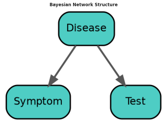

Cell 2.3: Independence from Structure¶

Network structure encodes independence: The visualization shows how graph structure represents conditional relationships
- Given Disease status, Symptom and Test observations become independent of each other
- This independence assumption is critical for efficient inference algorithms
- The graph structure encodes domain knowledge about relationships between variables

Part 3: Conditional Probability Tables (CPDs)¶

TODO(ai_gp): Replace CPD -> CPT¶

Cell 3.1: CPD Definition and Role¶

CPD: Conditional probability table assigns numerical beliefs to network structure
- Root nodes (no parents): Prior probability distribution
- Non-root nodes: Conditional probability given parent values
Medical domain knowledge encoded in CPDs:
- Disease prevalence in population
- Symptom likelihood given disease status
- Diagnostic test accuracy
Key concept: CPDs + network structure = complete probabilistic model
- Enables queries about unobserved variables given evidence

Cell 3.2: Interactive CPD Visualization¶

Goal: Explore how disease prevalence affects the joint conditional probability tables

Adjust disease prior probability and observe CPD updates
Understand relationship between prior belief and likelihood functions
Visualize how all three CPDs interact

Plots:

P(Disease): Prior probability of disease given current slider setting
P(Symptom | Disease): Conditional probability of symptom given disease state
P(Test | Disease): Conditional probability of test given disease state

Parameters:

Disease prior probability slider: ranges 0.0 to 1.0, affects P(Disease) heatmap
Disease state toggle: select None, Present, or Absent

Key observations:

Higher disease prior increases “Present” bar in first heatmap
CPD conditional probabilities stay constant; only priors change
Symptom and Test tables show likelihood of evidence given disease state

# Interactive CPD visualization

# TODO(ai_gp): Make the heatmaps use the same color scheme.
utils.cell3_2_create_cpd_widget(disease_prior=0.05)

# TODO(ai_gp): Add an explanation of what happens moving the P(Disease) and with the state toggle.

Part 4: Prior Distribution and Inference¶

Cell 4.1: Sampling from Prior¶

# Create medical network and sample from prior distribution.
model = utils.create_medical_network()

# Sample from the prior distribution using forward sampling.
samples = model.simulate(n_samples=1000, show_progress=False)

# Plot the samples and network structure.
utils.cell4_1_plot_forward_samples(samples)
plt.show()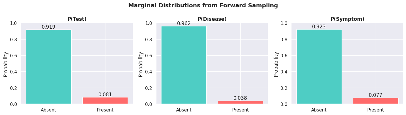

Sampling reveals prior beliefs: The distribution shows what the network believes in a vacuum without any observations
- Disease is rare (5% prior), so both Symptom and Test mostly indicate Absent status
- Base rate dominance: the rare disease prior overwhelms the samples
- Each sample represents one hypothetical patient drawn from the network’s generative model

Cell 4.2: Exact vs Approximate Inference¶

from pgmpy.inference import VariableElimination

# Create medical network.
model = utils.create_medical_network()

# Perform exact inference using Variable Elimination.
inference = VariableElimination(model)

# Compute exact marginal probabilities for each variable.
exact_results = {}
for var in model.nodes():
    exact_results[var] = inference.query(variables=[var])

# Generate samples from the network for comparison.
n_samples = 1000
samples = model.simulate(n_samples=n_samples, show_progress=False)

# Plot exact vs sampling comparison.
utils.cell4_2_plot_exact_vs_sampling(exact_results, samples)
plt.show()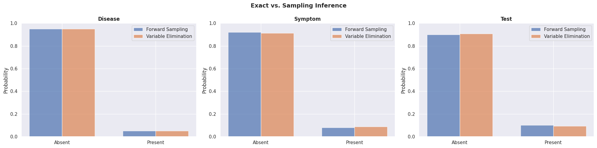

Exact inference vs forward sampling: Both methods answer what we believe about the prior distribution
- Exact results (blue line) computed with Variable Elimination, guaranteed correct
- Forward sampling results (orange) match exactly; accuracy improves with more samples
- Scaling comparison: Exact scales poorly as network grows (exponential), sampling scales better but needs many samples
Algorithm tradeoffs:
- Variable Elimination: Guaranteed correct, fast for small networks, intractable for large networks
- Forward Sampling: Approximate, scales to large networks, needs more samples for same accuracy

Part 5: Conditioning on Evidence¶

Cell 5.1: Effect of Evidence on Beliefs¶

# Create medical network and inference engine.
model = utils.create_medical_network()
inference = VariableElimination(model)

# Compute prior and posterior distributions.
prior = inference.query(variables=["Disease"])
posterior_pos = inference.query(
    variables=["Disease"], evidence={"Test": "Positive"}
)
posterior_neg = inference.query(
    variables=["Disease"], evidence={"Test": "Negative"}
)

# Plot belief updates from prior and posteriors.
utils.cell5_1_plot_belief_update(prior, posterior_pos, posterior_neg)
plt.show()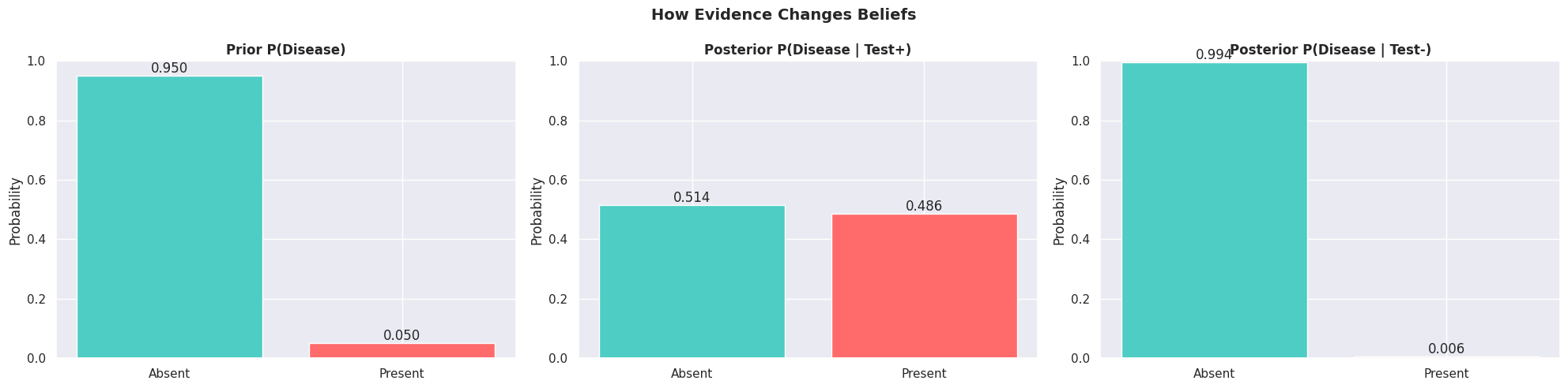

Bayes’ rule in action: Observing evidence shifts posterior probabilities away from prior beliefs
- Formula: $\Pr(\text{Disease} | \text{Evidence}) = \frac{\Pr(\text{Evidence} | \text{Disease}) \Pr(\text{Disease})}{\Pr(\text{Evidence})}$
- Positive test shifts disease probability from 5% (prior) to ~45% (posterior)
- Negative test dramatically reduces disease probability to <1%
Evidence informativeness: The strength of the shift depends on test accuracy and base rate
- Test is fairly informative: 95% sensitivity (true positive), 90% specificity (true negative)
- But base rate effect still matters: rare diseases stay rare unless evidence is overwhelming

Cell 5.2: Evidence Combination and Strength¶

# Create medical network.
model = utils.create_medical_network()

# Perform exact inference with evidence.
inference = VariableElimination(model)

# Compute exact marginals under evidence.
evidence = {"Test": "Positive"}
exact_results = {}
for var in model.nodes():
    exact_results[var] = inference.query(variables=[var], evidence=evidence)

# Generate samples under evidence.
n_samples = 1000
samples = model.simulate(n_samples=n_samples, evidence=evidence, show_progress=False)

# Plot exact vs sampling comparison under evidence.
utils.cell5_2_plot_exact_vs_sampling(exact_results, samples)
plt.show()

---------------------------------------------------------------------------
ValueError                                Traceback (most recent call last)
Cell In[9], line 11
      7 # Compute exact marginals under evidence.
      8 evidence = {"Test": "Positive"}
      9 exact_results = {}
     10 for var in model.nodes():
---> 11     exact_results[var] = inference.query(variables=[var], evidence=evidence)
     12 
     13 # Generate samples under evidence.
     14 n_samples = 1000

File /opt/venv/lib/python3.12/site-packages/pgmpy/inference/ExactInference.py:282, in VariableElimination.query(self, variables, evidence, virtual_evidence, elimination_order, joint, show_progress)
    280 common_vars = set(evidence if evidence is not None else []).intersection(set(variables))
    281 if common_vars:
--> 282     raise ValueError(
    283         f"Can't have the same variables in both `variables` and `evidence`. Found in both: {common_vars}"
    284     )
    286 if not variables:
    287     raise ValueError("The `variables` argument to query() must contain at least one variable.")

ValueError: Can't have the same variables in both `variables` and `evidence`. Found in both: {'Test'}

Core inference concept: Observing evidence shifts what we believe about unobserved variables
- Prior: Disease probability = 5%
- Positive test: Disease probability = ~45%
- Negative test: Disease probability = <1%
Strength of shift depends on evidence informativeness:
- Test accuracy: 95% for positives, 90% for negatives
- Fairly informative about disease status
Bayes’ rule in action: $\Pr(\text{Disease} | \text{Evidence}) = \frac{\Pr(\text{Evidence} | \text{Disease}) \Pr(\text{Disease})}{\Pr(\text{Evidence})}$
- Prior beliefs updated using observed evidence

Cell 5.3: Interactive Evidence Explorer¶

Goal: Understand how combining multiple evidence updates disease belief via Bayes’ rule

Observe posterior shifts as evidence combinations change
Discover how different evidence sources interact
Learn that order of evidence doesn’t matter

Plots:

Network structure visualization with evidence nodes highlighted
Posterior bar chart showing P(Disease | Evidence) distribution

Parameters:

Test Result dropdown: None, Positive, or Negative
Symptom dropdown: None, Present, or Absent
Clear Evidence button: resets both dropdowns

Key observations:

Positive test alone increases disease probability to 45%
Positive test + symptom present gives strongest evidence (~73%)
Positive test + symptom absent conflicts, reduces disease probability
Order of evidence combination doesn’t affect final posterior

# Interactive evidence explorer
model = utils.cell5_3_create_network()
utils.cell5_3_create_evidence_explorer()

Part 6: Inference Algorithm Comparison¶

Cell 6.1: Algorithm Comparison¶

import time
from pgmpy.inference import BeliefPropagation

# Create medical network.
model = utils.create_medical_network()
evidence = {"Test": "Positive"}

# Variable Elimination inference.
ve_inference = VariableElimination(model)
start = time.time()
ve_result = ve_inference.query(variables=["Disease"], evidence=evidence)
ve_time = (time.time() - start) * 1000
ve_probs = ve_result.values.flatten()

# Belief Propagation inference.
bp_inference = BeliefPropagation(model)
start = time.time()
bp_result = bp_inference.query(variables=["Disease"], evidence=evidence)
bp_time = (time.time() - start) * 1000
bp_probs = bp_result.values.flatten()

# Sampling-based inference.
start = time.time()
samples = model.simulate(
    n_samples=10000, evidence=evidence, show_progress=False
)
sampling_time = (time.time() - start) * 1000
sampling_result = (
    samples["Disease"].value_counts(normalize=True).sort_index()
)
sampling_probs = sampling_result.values

# Plot algorithm comparison results and timing.
utils.cell6_1_plot_algorithm_comparison(
    ve_probs, bp_probs, sampling_probs,
    ve_time, bp_time, sampling_time
)
plt.show()

Algorithm equivalence on small networks: All inference methods answer the same question correctly
- Variable Elimination: Exact, efficient for small networks
- Belief Propagation: Exact for tree networks, efficient structure exploitation
- Sampling (Forward, Gibbs): Approximate, more accurate with more samples
Practical algorithm selection:
- Small networks (<=15 variables): Use exact methods (Variable Elimination)
- Larger networks (>15 variables): Use approximate methods (Sampling, Variational Inference)
- Network topology matters: Tree networks have faster exact algorithms than general loopy networks

Inference algorithms: Different approaches with different performance tradeoffs
Exact methods:
- Variable Elimination: Efficient for small networks
- Belief Propagation: Efficient for tree-structured networks
Approximate methods:
- Sampling: Scales to large networks, requires more samples for accuracy
Small networks: All methods give identical results
- Choice of algorithm driven by network size and structure

Part 7: Advanced Topics¶

Cell 7.1: MAP Queries¶

# Create medical network and inference engine.
model = utils.create_medical_network()
inference = VariableElimination(model)

# Find MAP assignment given evidence.
evidence = {"Test": "Positive"}
map_result = inference.map_query(
    variables=["Disease", "Symptom"], evidence=evidence
)

# Compute full joint distribution for visualization.
joint_result = inference.query(
    variables=["Disease", "Symptom"], evidence=evidence
)

# Plot MAP result highlighting the most likely joint assignment.
utils.cell7_1_plot_map_result(map_result, joint_result)
plt.show()

MAP query finds single best explanation: Different from marginal inference which computes individual probabilities
- Marginal: $\Pr(\text{Disease} = \text{Yes} | \text{Evidence})$ for individual variables
- MAP: $\arg\max_{\text{all vars}} \Pr(\text{Disease}, \text{Symptom}, ... | \text{Evidence})$ single joint assignment
- Practical use: Diagnostics want single best explanation, not individual probability distributions
Interpretation: The result shows the joint state that maximizes posterior probability
- Most likely to occur given the evidence
- Useful when you need one actionable answer, not a full probability distribution
Distinction from marginal inference:
- Marginal: $\Pr(\text{Disease} = \text{Yes} | \text{Evidence})$ for individual variables
- MAP: $\arg\max \Pr(\text{Disease}, \text{Symptom} | \text{Evidence})$ single joint assignment
Practical use: Diagnostics want single best explanation
- “What’s most likely disease state and symptom combination?”

Cell 7.2: Gibbs Sampling Convergence¶

Goal: Visualize how MCMC sampling converges to true posterior and understand burn-in

Observe running mean trajectory over iterations
Understand burn-in period and why samples are discarded
Explore accuracy vs computational cost tradeoff

Plots:

Running mean trajectory: averaged probability estimate over iterations
Burn-in period shaded in gray: iterations discarded before convergence
True posterior line: reference value from exact inference
Confidence region: band around true posterior

Parameters:

Seed slider: control randomness of sampling chain (0-99)
N samples slider: total number of MCMC iterations (log scale 64-8192)
Burn-in slider: number of initial samples to discard (0-2000)

Key observations:

Running mean jumps early (initialization), then converges smoothly
Burn-in period visibly higher variability, settles after discard
Longer chains give smoother convergence curves
All chains converge to same true posterior regardless of seed

# Gibbs sampling interactive visualization
model = utils.cell7_2_create_network()
utils.cell7_2_gibbs_sampling_interactive()

Cell 7.3: Joint Distribution Explorer¶

Goal: Explore joint and marginal distributions under different evidence scenarios

Visualize full joint distribution as heatmap
Compare individual marginal distributions
Understand independence relationships in the network

Plots:

Joint distribution heatmap P(Disease, Symptom) with color intensity showing probability
Marginal bar charts: P(Disease) and P(Symptom) derived from joint

Parameters:

Disease dropdown: None, Present, or Absent (condition on disease evidence)
Symptom dropdown: None, Present, or Absent (condition on symptom evidence)

Key observations:

Joint heatmap shows all combinations; marginals sum across rows/columns
No evidence: heatmap reveals correlated structure (disease causes symptom)
Conditioning on disease: symptom distribution changes based on disease state
Different evidence combinations show different dependency structures

Part 8: Scaling to Larger Networks¶

Cell 8.1: Larger Network Interactive Demo¶

Goal: Compare inference algorithms on a realistic 8-variable network

Test Variable Elimination vs sampling on larger problem
Observe algorithm performance tradeoffs
Understand when approximation becomes necessary

Plots:

Network topology visualization with evidence nodes highlighted
Posterior disease probability bar chart with inference times

Parameters:

Scenario dropdown: choose evidence combinations (Test only, Test+Symptoms, Test but no Symptom)
Method dropdown: Variable Elimination or Sampling

Key observations:

Variable Elimination exact but slower on larger networks
Sampling approximation comparable speed with good accuracy
Same evidence produces consistent posteriors across methods
Network size and topology affect which algorithm to choose

Cell 8.2: Practical Workflow Demonstration¶

# Step 1: Load and inspect the network model.
model = utils.cell8_2_larger_network_demo()
_LOG.info("Model has %d nodes and %d edges", len(model.nodes()), len(model.edges()))
_LOG.info("Nodes: %s", list(model.nodes()))

# Validate the model.
model.check_model()
_LOG.info("Model validity: VALID")

# Step 2: Choose inference algorithm.
_LOG.info("\nFor an 8-node network: Variable Elimination is exact and fast")

# Step 3: Query the model with evidence.
evidence = {"Test1": "Positive", "Symptom1": "Present"}
_LOG.info("Evidence: %s", str(evidence))

# Perform inference using Variable Elimination.
inference = VariableElimination(model)
start = time.time()
result = inference.query(variables=["Disease"], evidence=evidence)
elapsed = (time.time() - start) * 1000
_LOG.info("\nResult P(Disease | Evidence):")
_LOG.info(str(result))
_LOG.info("Time: %.3f ms", elapsed)

# Step 4: Visualize and report results.
_LOG.info("\nStep 4: Visualize Results")
_LOG.info("=" * 50)

utils.cell8_2_plot_workflow_result(result)
plt.show()

_LOG.info(
    "\nConclusion: %.1f%% probability of disease given evidence",
    result.values.flatten()[1] * 100,
)

Practical workflow: From model to inference and interpretation
Steps:
1. Load pre-trained or pre-built Bayesian network
2. Inspect model structure and probability tables
3. Validate CPDs are well-formed (sum to 1)
4. Choose inference algorithm based on network size
5. Query with evidence to answer domain questions
6. Interpret results in context