Imports
%load_ext autoreload
%autoreload 2

import logging

import pandas as pd
import statsmodels.formula.api as smf
from IPython.display import display
The autoreload extension is already loaded. To reload it, use:
%reload_ext autoreload
import helpers.hnotebook as hnotebo
import helpers.hpandas_display as hpandisp
import helpers.hpandas_stats as hpanstat
import helpers.htutorial as ut
import L08_04_05_propensity_score_utils as mtl0psu

ut.config_notebook()

# Initialize logger.
logging.basicConfig(level=logging.INFO)
_LOG = logging.getLogger(__name__)
# Note: the original code called a non-existent `set_all_loggers_to_print()`
# top-level function; `init_loggers(..., set_all_loggers_to_print=True)` is
# the actual public API for what this was trying to do.
hnotebo.init_loggers(_LOG, set_all_loggers_to_print=True)

dir_name = "L08_data"
!ls $dir_name

out_dir_name = "figures/"
Part 1: Exploratory Analysis
Cell 1.1: Loading the management-training data
Goal:
- Load the manager-training dataset used throughout this notebook
The dataset contains information on managers with the following variables:
- intervention: binary treatment indicator (1 = received training, 0 = control)
- engagement_score: primary outcome: average standardized engagement score of the manager’s employees
- department_id: unique department identifier
- tenure: years the manager has been with the company
- n_of_reports: number of direct reports the manager has
- gender: manager’s identified gender (categorical)
- role: job category within the company (categorical)
- department_size: number of employees in the department
- department_score: average engagement score in the department
- last_engagement_score: previous period’s engagement score for the manager
df = pd.read_csv(f"{dir_name}/management_training.csv")
hpandisp.display_df(df)
pymc is not installed
arviz is not installed
preliz is not installed
sns is not installed
Python 3.12.13
Linux 3f3aef6a9c0f 6.12.67-linuxkit #1 SMP Sun Jan 25 02:26:28 UTC 2026 aarch64 GNU/Linux
Cell 1.2: Exploring distributions and correlations
Goal:
- Check the distribution of each variable, and how variables correlate with each other, before fitting any model
Implementation: hpanstat.explore_dataframe(df, ...)
show_distributions = True
show_correlations = True

hpanstat.explore_dataframe(
    df,
    show_distributions=show_distributions,
    show_correlations=show_correlations,
)
INFO:helpers.hpandas_stats:stats_df=
WARNING: Can't find pytz: continuing
INFO:helpers.hpandas_stats:Univariate distributions:
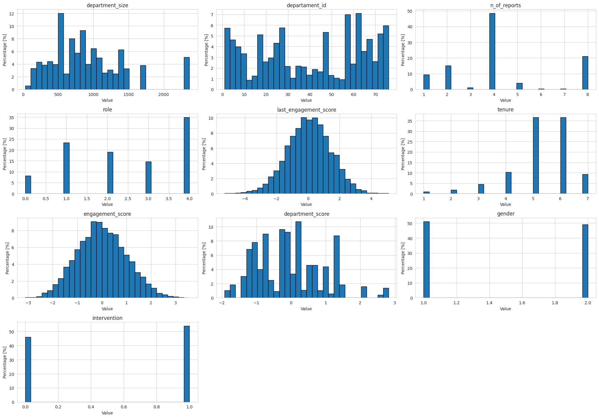
INFO:helpers.hpandas_stats:Correlation matrix:
Part 2: Naive Treatment Effect
Cell 2.1: Estimating the unadjusted average treatment effect
Goal:
- Estimate the treatment effect by regressing the outcome on the treatment indicator alone, ignoring all other covariates
Implementation: smf.ols("engagement_score ~ intervention", data=df)
model = smf.ols("engagement_score ~ intervention", data=df).fit()
print("ATE:", model.params["intervention"])
print("95% CI:", model.conf_int().loc["intervention", :].values.T)

display(model.summary().tables[1])
Cell 2.2: Visualizing engagement by treatment status
Goal:
- Visualize the raw relationship between treatment and outcome, both overall and split by department
Implementation: mtl0psu.plot_engagement_vs_intervention(df),
mtl0psu.plot_engagement_vs_intervention_by_department(df)
mtl0psu.plot_engagement_vs_intervention(df)ATE: 0.43459886274141496
95% CI: [0.39693035 0.47226738]
mtl0psu.plot_engagement_vs_intervention_by_department(df)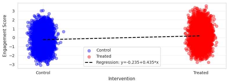
Cell 2.3: Visualizing every covariate by treatment status
Goal:
- Check whether the treated and control groups differ on any observed covariate, which would indicate confounding
Implementation: mtl0psu.plot_all_variables_density_by_intervention(df)
mtl0psu.plot_all_variables_density_by_intervention(df)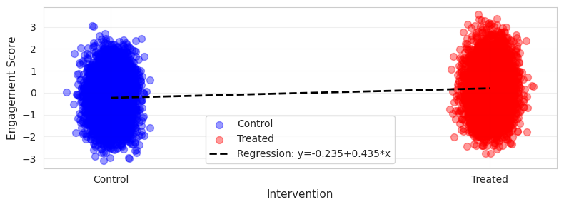
Cell 2.4: Adjusting for covariates
Goal:
- Re-estimate the treatment effect while adjusting for the observed covariates, to see how much the naive estimate was biased
Implementation:
smf.ols("engagement_score ~ intervention + tenure + ...", data=df)
# To reduce this bias, you can adjust for the covariates you have in your data.
model_adj = smf.ols(
    """
    engagement_score ~ intervention
        + tenure + last_engagement_score + department_score
        + n_of_reports + C(gender) + C(role)""",
    data=df,
).fit()

print("ATE (adjusted):", model_adj.params["intervention"])
print("95% CI (adjusted):", model_adj.conf_int().loc["intervention", :].values.T)
print("ATE (naive):", model.params["intervention"])
print("95% CI (naive):", model.conf_int().loc["intervention", :].values.T)
- The adjusted effect estimate is considerably smaller than the naive one
- This is some indication of positive bias: managers whose employees were already more engaged are more likely to have participated in the manager training program
Part 3: Propensity Score
Cell 3.1: Estimating the propensity score
Goal:
- Fit a propensity-score model, the probability of treatment given covariates, to later use as a single balancing score
Implementation: smf.logit("intervention ~ ...", data=df)
ps_model = smf.logit(
    """
    intervention ~
        tenure + last_engagement_score + department_score
        + C(n_of_reports) + C(gender) + C(role)""",
    data=df,
).fit(disp=0)

data_ps = df.copy()
data_ps["propensity_score"] = ps_model.predict(df)

display(data_ps[["intervention", "engagement_score", "propensity_score"]].head())
Cell 3.2: Adjusting for the propensity score directly
Goal:
- Use the propensity score itself as a single covariate, instead of the full covariate set, to adjust for confounding
# Estimate using propensity score as confounder / covariate.
model_ps = smf.ols(
    "engagement_score ~ intervention + propensity_score",
    data=data_ps,
).fit()
print("ATE (propensity-score covariate):", model_ps.params["intervention"])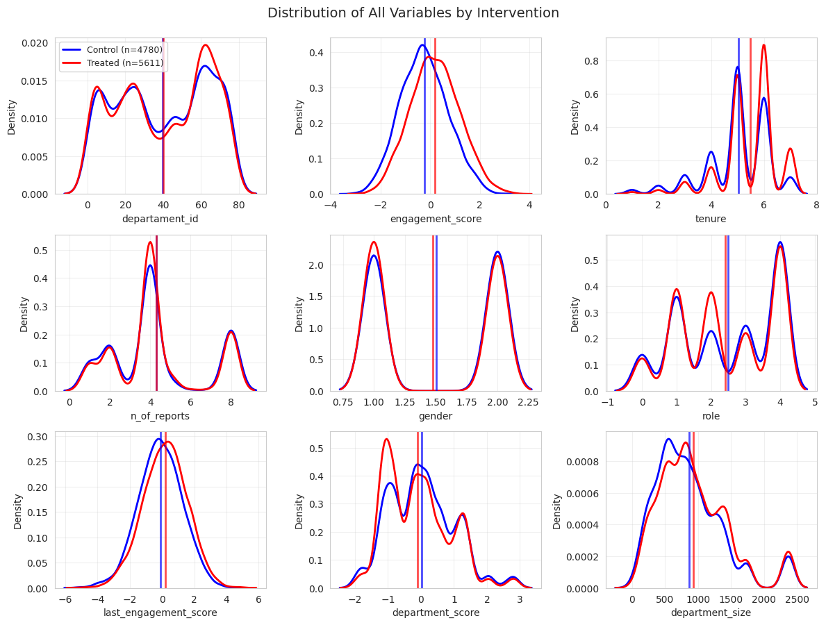
Part 4: Propensity Score Matching
Cell 4.1: Matching on the propensity score
Goal:
- Estimate the ATE by matching each treated unit to its nearest control unit (and vice versa) on the propensity score
Implementation: mtl0psu.propensity_score_matching(data_ps),
mtl0psu.calculate_psm_ate(predicted)
# Perform 1-nearest neighbor propensity score matching.
predicted = mtl0psu.propensity_score_matching(data_ps)
display(predicted.head())
ATE: 0.26779085766768607
95% CI: [0.23357751 0.30200421]
# Calculate average treatment effect from propensity score matching.
hat_ATE = mtl0psu.calculate_psm_ate(predicted)
print(f"ATE (propensity score matching): {hat_ATE:.4f}")
ATE: 0.43459886274141496
95% CI: [0.39693035 0.47226738]
Cell 4.2: Inverse probability of treatment weighting
Goal:
- Estimate the ATE by reweighting units by the inverse of their propensity score, instead of matching
Implementation: mtl0psu.plot_iptw(data_ps),
mtl0psu.estimate_ate_iptw(data_ps)
# Plot inverse probability of treatment weighting results.
mtl0psu.plot_iptw(data_ps)
# Estimate ATE using IPTW.
weighted_e_y1, weighted_e_y0, hat_ATE = mtl0psu.estimate_ate_iptw(data_ps)
print("E[Y1]:", weighted_e_y1)
print("E[Y0]:", weighted_e_y0)
print("ATE:", hat_ATE)Part 5: Variance of the IPW Estimator
Cell 5.1: Estimating the ATE with bootstrap confidence intervals
Goal:
- Quantify the uncertainty of the IPW estimator via bootstrap resampling, since it has no simple closed-form standard error
Implementation: mtl0psu.estimate_ate_with_ps(...),
mtl0psu.estimate_confidence_interval_bootstrap(...)
# Prepare formula and variables for IPW estimation.
formula = """
tenure + last_engagement_score + department_score
    + C(n_of_reports) + C(gender) + C(role)
"""
treatment_col = "intervention"
outcome_col = "engagement_score"
# Estimate ATE using IPW estimator.
ate_ipw = mtl0psu.estimate_ate_with_ps(
df, formula, treatment_col=treatment_col, outcome_col=outcome_col
)
print(f"ATE (IPW): {ate_ipw:.4f}")# Compute bootstrap 95% confidence interval for ATE using IPW.
est_fn = lambda data: mtl0psu.estimate_ate_with_ps(
data,
ps_formula=formula,
treatment_col=treatment_col,
outcome_col=outcome_col,
)
ci = mtl0psu.estimate_confidence_interval_bootstrap(
df, est_fn, rounds=200, seed=123, n_jobs=4, pcts=[2.5, 97.5]
)
print(f"ATE: {ate_ipw:.4f}")
print(f"95% confidence interval: {ci}")Part 6: Stabilized Propensity Weights
Cell 6.1: Checking the pseudo-population sample sizes
Goal:
- Check how many “effective” units the IPTW pseudo-population represents for each group, since extreme propensity scores can inflate a few units’ weight far beyond their actual count
# Show sample sizes for original and pseudo-population.
print("Original sample size:", data_ps.shape[0])

# Compute sample sizes after IPTW weighting.
treated = data_ps.query("intervention==1")
control = data_ps.query("intervention==0")

weight_t = 1 / treated["propensity_score"]
weight_nt = 1 / (1 - control["propensity_score"])

print("Treated pseudo-population sample size:", sum(weight_t))
print("Untreated pseudo-population sample size:", sum(weight_nt))
Cell 6.2: Estimating the ATE with stabilized weights
Goal:
- Re-estimate the ATE with stabilized weights, which rescale by the marginal treatment probability to reduce the influence of extreme propensity scores
Implementation: mtl0psu.estimate_ate_stabilized_weights(data_ps),
mtl0psu.plot_propensity_distributions(data_ps)
# Estimate ATE using stabilized propensity weights.
ate_stabilized = mtl0psu.estimate_ate_stabilized_weights(data_ps)
print(f"ATE (stabilized weights): {ate_stabilized:.4f}")
# Plot propensity score distributions before and after weighting.
mtl0psu.plot_propensity_distributions(data_ps)