Metalearners - MSML610 -- Tutorials

Imports¶

%load_ext autoreload
%autoreload 2

import logging

from matplotlib import pyplot as plt
import numpy as np
import pandas as pd
import seaborn as sns

try:
    from IPython.display import display
except ImportError:
    display = print  # type: ignore

import helpers.hdbg as hdbg
import helpers.hnotebook as hnotebo

import helpers.htutorial as ut
import L08_04_07_metalearners_utils as mtl

ut.config_notebook()

# Initialize logger.
logging.basicConfig(level=logging.INFO)
_LOG = logging.getLogger(__name__)
hnotebo.init_loggers(_LOG, set_all_loggers_to_print=True)

pymc is not installed
arviz is not installed
preliz is not installed
sns is not installed

Python 3.12.13
Linux 3a71c0a7bf16 6.12.67-linuxkit #1 SMP Sun Jan 25 02:26:28 UTC 2026 aarch64 GNU/Linux

import warnings

import helpers.hmodule as hmodule
from lightgbm import LGBMRegressor

warnings.filterwarnings("ignore", category=UserWarning, module="lightgbm")
warnings.filterwarnings(
    "ignore",
    message="X does not have valid feature names",
    category=UserWarning,
)
logging.getLogger("lightgbm").setLevel(logging.ERROR)

# `lightgbm`/`fklearn` are extras for this notebook, not in the shared
# requirements.txt, so they are self-installed here (see `mtl` for the
# `fklearn` usage).
hmodule.install_module_if_not_present(
    ["lightgbm", "fklearn"],
    use_activate=True,
    use_sudo=False,
    venv_path="/opt/venv",
)

Module 'lightgbm' is already installed.
Module 'fklearn' is already installed.

Part 1: Loading Data¶

Cell 1.1: Loading the email marketing datasets¶

Goal:

Load a biased (observational) and a randomized email marketing dataset, sharing the same schema, used throughout the T/X-Learner sections

dir_name = "L08_data"
!ls $dir_name

out_dir_name = "figures/"

data_biased = pd.read_csv(f"{dir_name}/email_obs_data.csv")
print("# data_biased")
print("num_rows=", len(data_biased))
display(data_biased.head())

data_rnd = pd.read_csv(f"{dir_name}/email_rnd_data.csv")
print("# data_rnd")
print("num_rows=", len(data_rnd))
display(data_rnd.head())

# data_biased
num_rows= 300000

# data_rnd
num_rows= 10000

hdbg.dassert_eq(data_biased.columns.tolist(), data_rnd.columns.tolist())

y = "next_mnth_pv"
T = "mkt_email"
X = list(data_rnd.drop(columns=[y, T]).columns)

train, test = data_biased, data_rnd

display(train[[T, y]].head())

Part 2: T-Learner¶

Cell 2.1: Fitting separate outcome models per treatment arm¶

Goal:

Fit one outcome model on the control arm and one on the treated arm, the T-Learner’s defining idea, then predict the CATE as their difference

Implementation:

m0/m1 are LGBMRegressor models fit on T==0/T==1 rows respectively; cate = m1.predict(x) - m0.predict(x)

np.random.seed(123)

m0 = LGBMRegressor()
m1 = LGBMRegressor()

m0.fit(train.query(f"{T}==0")[X].values, train.query(f"{T}==0")[y].values)
_ = m1.fit(train.query(f"{T}==1")[X].values, train.query(f"{T}==1")[y].values)

display(m0)

Cell 2.2: Evaluating the T-Learner CATE with a gain curve¶

Goal:

Check the T-Learner’s CATE estimate on the held-out randomized data, via a cumulative gain curve

Implementation: mtl.plot_gain_curve_analysis(cate_test, T, y, ...)

t_learner_cate_test = test.assign(
    cate=m1.predict(test[X].values) - m0.predict(test[X].values)
)

_ = mtl.plot_gain_curve_analysis(t_learner_cate_test, T, y, title="T-Learner")

[LightGBM] [Info] Auto-choosing row-wise multi-threading, the overhead of testing was 0.005163 seconds.
You can set `force_row_wise=true` to remove the overhead.
And if memory is not enough, you can set `force_col_wise=true`.
[LightGBM] [Info] Total Bins 548
[LightGBM] [Info] Number of data points in the train set: 146759, number of used features: 25
[LightGBM] [Info] Start training from score 88.249324
[LightGBM] [Info] Auto-choosing row-wise multi-threading, the overhead of testing was 0.004607 seconds.
You can set `force_row_wise=true` to remove the overhead.
And if memory is not enough, you can set `force_col_wise=true`.
[LightGBM] [Info] Total Bins 550
[LightGBM] [Info] Number of data points in the train set: 153241, number of used features: 25
[LightGBM] [Info] Start training from score 1596.224063

Cell 2.3: Visualizing treatment-effect heterogeneity on synthetic data¶

Goal:

Fit the same T-Learner pattern on synthetic data with a known, heterogeneous treatment effect, to visualize what the 2 outcome models and the resulting CATE actually look like

Implementation: mtl.generate_synthetic_treatment_data(...), mtl.fit_tlearner_models(...), mtl.plot_tlearner_treatment_effect_analysis(...)

# Generate synthetic data with treatment heterogeneity.
df = mtl.generate_synthetic_treatment_data(n0=500, n1=50, seed=123)

# Fit separate outcome models for control and treatment groups.
m0, m1, m0_hat, m1_hat = mtl.fit_tlearner_models(df, min_child_samples=25)

# Visualize outcome models and heterogeneous treatment effects.
mtl.plot_tlearner_treatment_effect_analysis(df, m0, m1, m0_hat, m1_hat)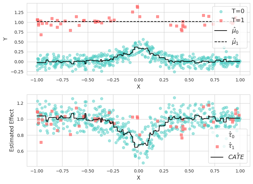

Part 3: X-Learner¶

Cell 3.1: Estimating heterogeneous treatment effects¶

Goal:

Compute the X-Learner’s imputed treatment effects: for each unit, the difference between its observed outcome and the other arm’s predicted outcome

Implementation:

mtl.calculate_xlearner_heterogeneous_treatment_effects(df, m0, m1)

tau_0, tau_1 = mtl.calculate_xlearner_heterogeneous_treatment_effects(df, m0, m1)

Cell 3.2: Fitting X-Learner second-stage models on synthetic data¶

Goal:

Fit a second-stage model on each arm’s imputed effects, then compare the resulting CATE estimates against the ground truth

Implementation: mtl.fit_xlearner_models(df, tau_0, tau_1, ...), mtl.plot_xlearner_effect_estimates(...)

mu_tau0, mu_tau1, mu_tau0_hat, mu_tau1_hat = mtl.fit_xlearner_models(
    df, tau_0, tau_1, min_child_samples=25
)

# Plot heterogeneous treatment effect estimates.
mtl.plot_xlearner_effect_estimates(df, tau_0, tau_1, mu_tau0_hat, mu_tau1_hat)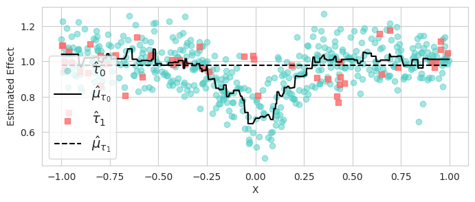

Cell 3.3: Visualizing propensity-score-weighted CATE¶

Goal:

Combine the 2 second-stage estimates into a single CATE, weighted by the propensity score, and visualize the result

Implementation: mtl.plot_xlearner_with_propensity_scores(...)

mtl.plot_xlearner_with_propensity_scores(df, mu_tau0, mu_tau1, tau_0, tau_1)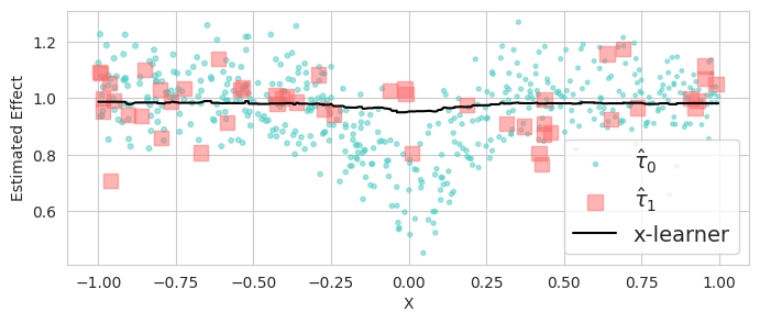

Cell 3.4: Fitting the propensity-score-weighted X-Learner on real data¶

Goal:

Repeat the X-Learner pattern on the real email data: first-stage models weighted by the inverse propensity score, then second-stage models on the residual treatment effects

Implementation:

mtl.fit_propensity_score_and_weighted_outcome_models(train, X, T, y)
mtl.fit_xlearner_second_stage_models(train, X, T, y, m0, m1)

# Fit propensity score model and first-stage outcome models with inverse
# probability weighting.
ps_model, m0, m1 = mtl.fit_propensity_score_and_weighted_outcome_models(
    train, X, T, y
)

# Fit second-stage models on residual treatment effects.
m_tau_0, m_tau_1 = mtl.fit_xlearner_second_stage_models(train, X, T, y, m0, m1)

Cell 3.5: Evaluating the X-Learner CATE with a gain curve¶

Goal:

Check the X-Learner’s CATE estimate on the held-out data, via the same cumulative gain curve used for the T-Learner

x_cate_test = mtl.estimate_xlearner_cate(test, X, ps_model, m_tau_0, m_tau_1)

_ = mtl.plot_gain_curve_analysis(x_cate_test, T, y, title="X-Learner")

Part 4: S-Learner¶

Cell 4.1: Loading the discount dataset¶

Goal:

Load a continuous-treatment dataset (discount level, not a binary flag), split chronologically into train/test

data_cont = pd.read_csv(f"{dir_name}/discount_data.csv")
print("data_cont.shape[0]=", data_cont.shape[0])
display(data_cont.head())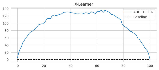

train = data_cont.query("day<'2018-01-01'")
print("train.shape[0]=", train.shape[0])
test = data_cont.query("day>='2018-01-01'")
print("test.shape[0]=", test.shape[0])

Cell 4.2: Fitting a single shared-covariate model¶

Goal:

Fit one model with treatment as a plain input feature (the S-Learner pattern), instead of 2 separate per-arm models

Implementation: mtl.fit_slearner_model(train, X, T, y)

X = ["month", "weekday", "is_holiday", "competitors_price"]
T = "discounts"
y = "sales"

s_learner = mtl.fit_slearner_model(train, X, T, y)

Cell 4.3: Generating counterfactual predictions¶

Goal:

Sweep the discount level through a grid of counterfactual values, to see how predicted sales respond

Implementation:

mtl.generate_slearner_counterfactual_predictions(test, X, T, y, s_learner, discount_grid)

test_cf = mtl.generate_slearner_counterfactual_predictions(
    test, X, T, y, s_learner, np.array([0, 10, 20, 30, 40])
)

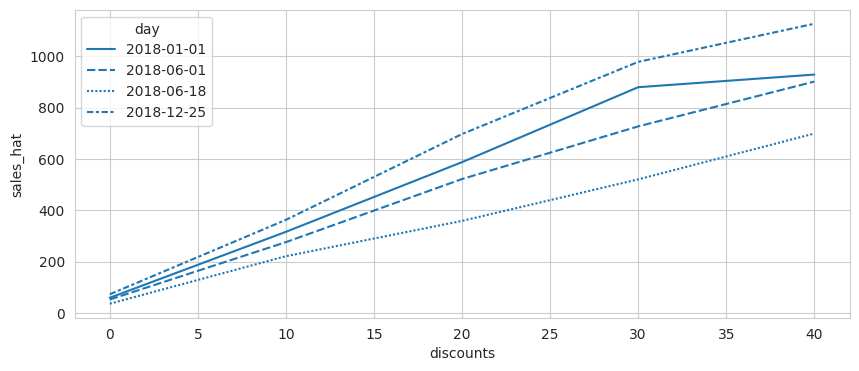
display(test_cf.head(8))

Cell 4.4: Visualizing counterfactual sales curves¶

Goal:

Plot the predicted sales-vs-discount curve for a few selected days, for one restaurant, to see how the shape varies day to day

days = ["2018-12-25", "2018-01-01", "2018-06-01", "2018-06-18"]

plt.figure(figsize=(10, 4))
_ = sns.lineplot(
    data=test_cf.query("day.isin(@days)").query("rest_id==2"),
    y="sales_hat",
    x="discounts",
    style="day",
)

Cell 4.5: Evaluating the S-Learner CATE with a gain curve¶

Goal:

Estimate the CATE from the counterfactual predictions, then check it with the same cumulative gain curve used for the T/X-Learners

Implementation: mtl.estimate_slearner_cate(test_cf, test, T, y)

test_s_learner_pred = mtl.estimate_slearner_cate(test_cf, test, T, y)

display(test_s_learner_pred.head())

_ = mtl.plot_gain_curve_analysis(test_s_learner_pred, T, y, title="S-Learner")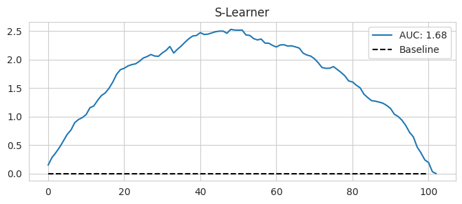

Part 5: Double ML / R-Learner¶

Cell 5.1: Fitting the debiasing and denoising nuisance models¶

Goal:

Fit the 2 nuisance models the R-Learner needs: one predicting treatment from covariates (debiasing), one predicting outcome from covariates alone (denoising)

Implementation: mtl.fit_rlearner_models(train, X, T, y)

X = ["month", "weekday", "is_holiday", "competitors_price"]
T = "discounts"
y = "sales"

# Fit debiasing and denoising models.
debias_m, denoise_m = mtl.fit_rlearner_models(train, X, T, y)

Cell 5.2: Fitting the R-Learner CATE model on residuals¶

Goal:

Regress the outcome residual on the treatment residual (both from the nuisance models above), whose slope is the R-Learner’s CATE estimate

Implementation: mtl.fit_rlearner_cate_model(train, X, T, y, debias_m, denoise_m)

cate_model, t_res, y_res = mtl.fit_rlearner_cate_model(
    train, X, T, y, debias_m, denoise_m
)

Cell 5.3: Checking coefficients via an OLS diagnostic¶

Goal:

Cross-check the R-Learner’s residual-on-residual regression against a plain OLS fit, as an optional diagnostic

import statsmodels.api as sm

display(sm.OLS(y_res, t_res).fit().summary().tables[1])

Cell 5.4: Evaluating the R-Learner CATE with a gain curve¶

Goal:

Estimate the CATE on the test set, then check it with the same cumulative gain curve used for the other 3 metalearners

test_r_learner_pred = mtl.estimate_rlearner_cate(test, X, cate_model)

_ = mtl.plot_gain_curve_analysis(test_r_learner_pred, T, y, title="R-Learner")