g-h filter - MSML610 -- Tutorials

Imports¶

%load_ext autoreload
%autoreload 2

import logging

import numpy as np
from IPython.display import display

import helpers.htutorial as ut

ut.config_notebook()

# Initialize logger.
logging.basicConfig(level=logging.INFO)
_LOG = logging.getLogger(__name__)

WARNING (pytensor.tensor.blas): Using NumPy C-API based implementation for BLAS functions.
vim support installed: restart the notebook, if needed

Python 3.12.3
Linux 589569fe8102 6.12.67-linuxkit #1 SMP Sun Jan 25 02:26:28 UTC 2026 aarch64 aarch64 aarch64 GNU/Linux

import helpers.hio as hio
import L09_04_gh_filter_utils as time_ut

dst_dir = "figures"
hio.create_dir(dst_dir, incremental=True)
!cp msml610/tutorials/figures/*.png msml610/lectures_source/figures

Part 1: Estimating Body Weight¶

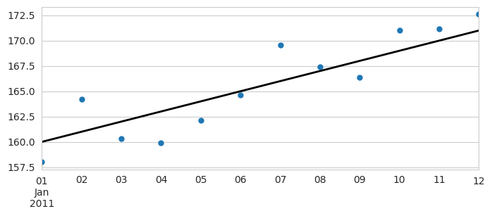
Cell 1.1: Ground truth vs measurements¶

Goal:

Look at a weight-measurement series against the (in practice unknown) ground truth, before fitting any filter to it

Implementation:

time_ut.cell1_1_plot_ground_truth_and_measurements(...)

n_samples = 12

# We assume we know the real weight.
ground_truth = 160.0 + np.arange(0, n_samples)

# This is what we measure.
measured_weights = np.array(
    [
        158.0,
        164.2,
        160.3,
        159.9,
        162.1,
        164.6,
        169.6,
        167.4,
        166.4,
        171.0,
        171.2,
        172.6,
    ]
)

df = time_ut.cell1_1_plot_ground_truth_and_measurements(
    measured_weights, ground_truth, dst_dir, "L09_04_ground_truth.png"
)
display(df.head())

Cell 1.2: Knowing the gain rate¶

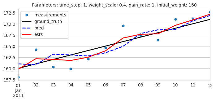
Goal:

Filter the measurements with the g-h filter’s internal model set to the correct gain rate, and check how closely it tracks the truth

Implementation: time_ut.cell1_2_plot_gh_filter_with_known_gain_rate

predict_using_gain_guess() predicts via weight + gain_rate * time_step, then blends the prediction with the measurement by weight_scale

params = {
    # This is the time interval between measurements.
    "time_step": 1,
    # This is the blending factor.
    "weight_scale": 4 / 10.0,
    # This is the internal model (ground truth).
    "gain_rate": 1.0,
    # This is the initial weight.
    "initial_weight": 160.0,
}
file_name = "L09_04_knowing_gain_rate.png"
time_ut.cell1_2_plot_gh_filter_with_known_gain_rate(
    measured_weights, ground_truth, params, dst_dir, file_name
)

Cell 1.3: Wrong guess of the gain rate¶

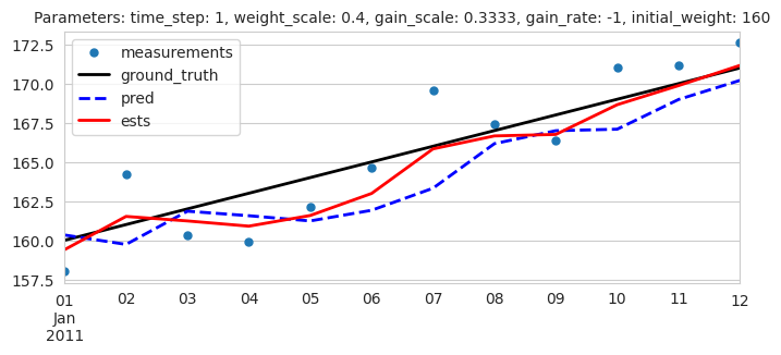
Goal:

Refit with a badly wrong gain-rate guess, to see how the filter’s tracking degrades when its internal model is wrong

params = {
    # This is the time interval between measurements.
    "time_step": 1,
    # This is the blending factor.
    "weight_scale": 4 / 10.0,
    # This is the internal model (wrong guess).
    "gain_rate": -10.0,
    # This is the initial weight.
    "initial_weight": 160.0,
}
file_name = "L09_04_wrong_gain_rate.png"
time_ut.cell1_3_plot_gh_filter_with_known_gain_rate(
    measured_weights, ground_truth, params, dst_dir, file_name
)

Cell 1.4: Interactively exploring the gain rate¶

Goal:

Let students sweep the initial weight, blending factor, and gain rate by hand, to build intuition for how each one shapes the fit

Implementation: time_ut.cell1_4_create_interactive_gain_rate_widget()

time_ut.cell1_4_create_interactive_gain_rate_widget(
    measured_weights, ground_truth
)

Usage

Inputs
- weight: initial weight estimate
- weight_scale: blending factor between prediction and measurement
- gain_rate: assumed rate of weight gain per time step
Panels
- left: measurements, ground truth, predictions, and estimates
- Comments: the current parameters, and the final estimate’s error against the ground truth

Guided usage

Set gain_rate far from 1.0 (the true value)
- Observe the final |error| in Comments grows
Slide gain_rate back toward 1.0
- Observe the estimate line converges back onto the ground truth

Cell 1.5: Learning the gain rate¶

Goal:

Let the filter itself update its gain-rate guess from the residual at each step, instead of relying on a fixed guess

Implementation:

time_ut.cell1_5_plot_gh_filter_with_learning_gain_rate
predict_learning_gain_rate() updates gain_rate by gain_scale * residual / time_step at every step

params = {
    # Time interval between measurements.
    "time_step": 1,
    # Scale for updating the weight estimate (blending factor).
    "weight_scale": 4 / 10.0,
    # Scale for updating the gain rate estimate.
    "gain_scale": 1 / 3.0,
    # Initial guess for the gain rate.
    "gain_rate": -1.0,
    # Initial value for weight estimate.
    "initial_weight": 160.0,
}
file_name = "L09_04_learning_gain_rate.png"

time_ut.cell1_5_plot_gh_filter_with_learning_gain_rate(
    measured_weights, ground_truth, params, dst_dir, file_name
)

Part 2: g-h Filter on Noisy Measurements¶

Cell 2.1: Interactively exploring noisy linear data¶

Goal:

Let students see how the seed, sample count, and noise level shape a synthetic linear-plus-noise series, before filtering it

Implementation:

time_ut.cell2_1_create_interactive_linear_noisy_data_widget()

time_ut.cell2_1_create_interactive_linear_noisy_data_widget()

Usage

Inputs
- seed: random seed for the noise
- count: number of points to generate
- noise_factor: standard deviation of the additive noise
Panels
- left: the noisy measurements against the noiseless ground truth
- Comments: the current parameters, and the residual mean/std dev between measurements and ground truth

Guided usage

Raise noise_factor from 0 toward its max
- Observe the residual std dev in Comments grows roughly linearly with it

Cell 2.2: Correct initial guess¶

Goal:

Filter noisy data with initial guesses that match the true system, as a baseline for the wrong-guess case in Cell 2.3

Implementation: time_ut.cell2_2_plot_gh_filter_with_params(params)

# Demonstrate g-h filter with correct initial guesses.
params = {
    # Initial guesses (actually correct!).
    "x0": 0,
    "dx": 1,
    "dt": 1,
    "g": 0.1,
    "h": 0.02,
}
time_ut.cell2_2_plot_gh_filter_with_params(params)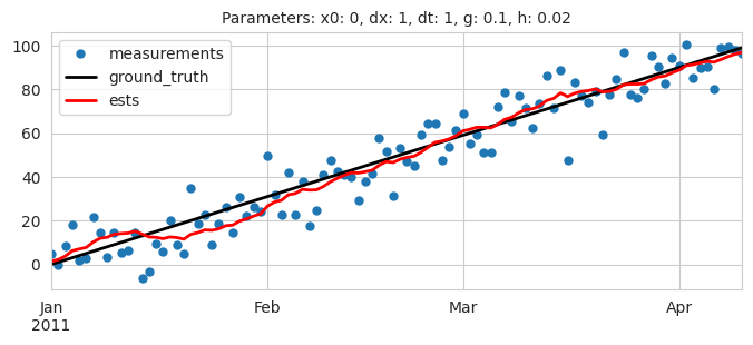

Cell 2.3: Wrong initial guess¶

Goal:

Refit with wrong initial guesses, to see how much the filter still recovers thanks to the correcting effect of the measurements

# Demonstrate g-h filter with wrong initial guesses.
params = {
    # Initial guesses (wrong!).
    "x0": 100,
    "dx": 2,
    "dt": 1,
    "g": 0.2,
    "h": 0.02,
}
time_ut.cell2_3_plot_gh_filter_with_params(params)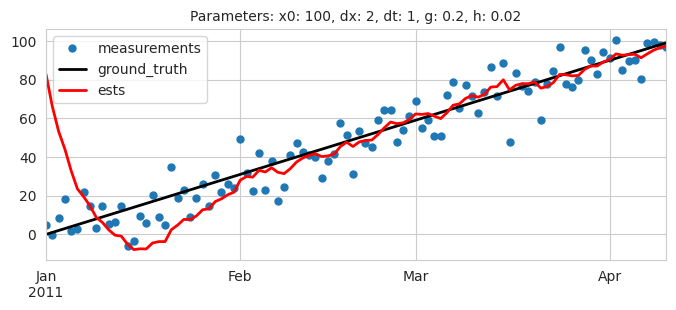

Cell 2.4: Extreme noise¶

Goal:

Check how the filter degrades as the noise level grows far beyond what Cells 2.2/2.3 used

Implementation: time_ut.cell2_4_extreme_noise()

time_ut.cell2_4_extreme_noise()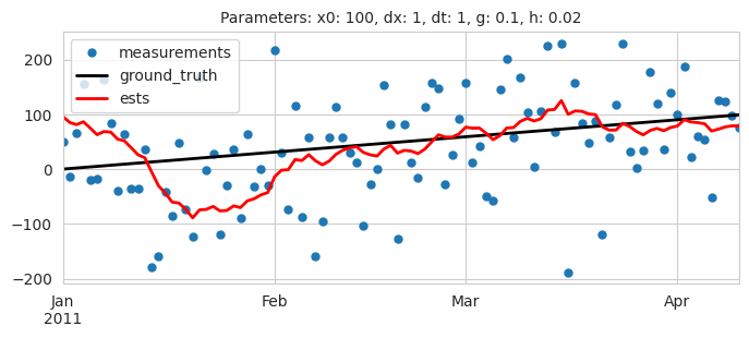

Cell 2.5: Interactively exploring non-linear noisy data¶

Goal:

Let students see how adding acceleration to the generating process changes the data, since the g-h filter assumes constant velocity

Implementation:

time_ut.cell2_5_create_interactive_non_linear_noisy_data_widget()

time_ut.cell2_5_create_interactive_non_linear_noisy_data_widget()

Usage

Inputs
- seed: random seed for the noise
- count: number of points to generate
- noise_factor: standard deviation of the additive noise
- accel: acceleration of the underlying process
Panels
- left: the noisy measurements against the accelerating ground truth
- Comments: the current parameters, and the residual mean/std dev between measurements and ground truth

Guided usage

Set accel=0
- Observe the ground truth becomes a straight line, the constant- velocity case the g-h filter is designed for
Raise accel away from 0
- Observe the ground truth curves: a constant-velocity filter will systematically lag behind it

Cell 2.6: Non-linear data with the g-h filter¶

Goal:

Apply the (constant-velocity) g-h filter to the accelerating data from Cell 2.5, to see the systematic lag predicted there

Implementation: time_ut.cell2_6_non_linear_gh_filter()

time_ut.cell2_6_non_linear_gh_filter()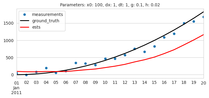

Cell 2.7: Varying g¶

Goal:

Compare 3 values of g on the same noisy data, and on a step-like signal, to see the tradeoff between smoothing and responsiveness

Implementation: time_ut.cell2_7_plot_varying_g_noisy(...), time_ut.cell2_7_plot_varying_g_step(...)

If g is smaller we follow more our model than the measurements
If g is larger we follow more the measurements than our model
If g is too large we follow the measurements and reject no noise

time_ut.cell2_7_plot_varying_g_noisy(dst_dir, "L09_04_varying_g1.png")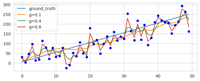

# If g is large we follow more the measures than our model.
time_ut.cell2_7_plot_varying_g_step(dst_dir, "L09_04_varying_g2.png")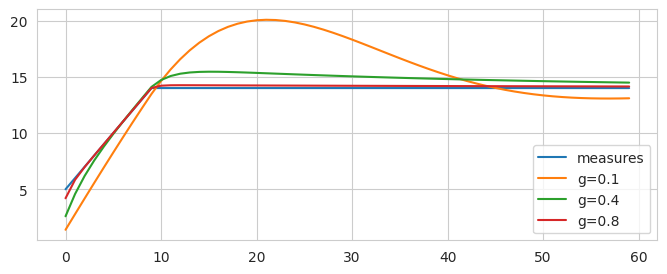

Cell 2.8: Varying h¶

Goal:

Compare 3 (dx, h) combinations on a ramp signal, to see how h trades off ringing amplitude against adaptation speed

Implementation: time_ut.cell2_8_plot_varying_h(dst_dir, ...)

h affects how much we favor the measurement of $\frac{dx}{dt}$ vs our prediction
If the signal is varying a lot, then we will react to the transient rapidly

time_ut.cell2_8_plot_varying_h(dst_dir, "L09_04_varying_h1.png")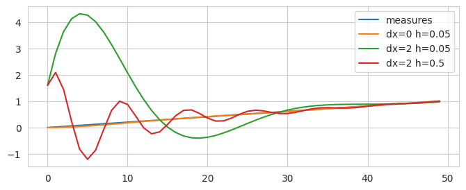

Cell 2.9: Interactively exploring the g-h filter¶

Goal:

Let students sweep every g-h filter parameter, plus the noise level, at once, to consolidate the intuition built in Cells 2.2-2.8

Implementation: time_ut.cell2_9_create_interactive_gh_filter_widget()

time_ut.cell2_9_create_interactive_gh_filter_widget()

Usage

Inputs
- x: initial state estimate
- dx: initial rate-of-change estimate
- g: state gain
- h: rate gain
- noise_factor: standard deviation of the additive noise
Panels
- left: ground truth, noisy measurements, and filtered estimates
- Comments: the current parameters, and the RMSE between the estimate and the ground truth

Guided usage

Set x/dx far from the data’s true start (5, 5)
- Observe the RMSE in Comments is high at first, then drops as the filter converges
Raise noise_factor to its max
- Observe the RMSE grows, and the estimate line gets visibly noisier