Imports
%load_ext autoreload
%autoreload 2

import logging

import numpy as np

import helpers.hintrospection as hintros
import helpers.htutorial as ut

ut.config_notebook()

# Initialize logger.
logging.basicConfig(level=logging.INFO)
_LOG = logging.getLogger(__name__)
WARNING (pytensor.tensor.blas): Using NumPy C-API based implementation for BLAS functions.
vim support installed: restart the notebook, if needed
Python 3.12.3
Linux 7d77d2247121 6.12.67-linuxkit #1 SMP Sun Jan 25 02:26:28 UTC 2026 aarch64 aarch64 aarch64 GNU/Linux
import helpers.hio as hio
import L09_05_02_univariate_kalman_filter_utils as time_ut

dst_dir = "figures"
hio.create_dir(dst_dir, incremental=True)
!cp msml610/tutorials/figures/*.png msml610/lectures_source/figures
Part 1: Sum and Product of Gaussians
Cell 1.1: Representing a Gaussian
Goal:
- Introduce
time_ut.Gaussian(mean, var), the(mean, var)named tuple used to represent a belief throughout this notebook
x = time_ut.Gaussian(3.4, 10.1)
print("x=", x)
print("x.mean=", x.mean)
print("x.var=", x.var)
N(mu=3.400, sigma^2=10.100)
x.mean= 3.4
x.var= 10.1
Cell 1.2: Sum of Gaussians
- Given 2 Gaussians and
- For correlated Gaussians with correlation coefficient , the sum is a Gaussian with:
- Interpretation:
- The mean is the sum of the means (by linearity)
- For independent Gaussians (), the variance is the sum of variances (uncertainty increases)
- Positive correlation increases variance, negative correlation decreases it
Implementation: time_ut.gaussian_sum(x, y)
# Sum two Gaussians.
x = time_ut.Gaussian(10, 0.2**2)
y = time_ut.Gaussian(15, 0.7**2)

z = time_ut.gaussian_sum(x, y)
print("z=", z)
N(mu=25.000, sigma^2=0.530)
ax = time_ut.plot_gaussian(x, label="x")
time_ut.plot_gaussian(y, ax=ax, label="y")
_ = time_ut.plot_gaussian(z, ax=ax, label="z")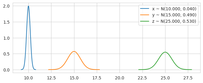
Implementation: time_ut.cell1_1_plot_gaussian_sum()
- Plots input Gaussians (blue) and (yellow) as filled PDFs, the analytical sum (red line), and a numerical sum via sampling (light coral histogram)
hintros.print_obj_info(time_ut.cell1_1_plot_gaussian_sum)time_ut.cell1_1_plot_gaussian_sum()Usage
Inputs
mu1(): mean ofsigma1(): standard deviation ofmu2(): mean ofsigma2(): standard deviation ofrho(): correlation coefficient between and
Panels
left: and as filled PDFs, the analytical sum , and the sampled numerical sum
Guided usage
- Set
rho=0- Observe ’s variance equals exactly
- Raise
rhotoward1- Observe ’s variance grows beyond
- Lower
rhotoward-1- Observe ’s variance shrinks below
- In every case, observe ’s mean stays
Cell 1.3: Product of Gaussians
- Given 2 Gaussians and
- The product (PDF multiplication) is a Gaussian with:
- Interpretation:
- Reduces variance by incorporating more information
- If one Gaussian is narrower (more accurate), the result leans towards
- If the 2 Gaussians are similar (measures corroborate), the result becomes more certain
Gaussian products in terms of precision
The precision of a Gaussian is
The precision of the product is the sum of the precisions
The mean is the average of the means weighted by the precisions
The mean is averaged towards the more certain Gaussian
The variance is smaller than both
Implementation: time_ut.gaussian_multiply(x, y)
# Product of two equal Gaussians.
x = time_ut.Gaussian(10, 1.0)

z = time_ut.gaussian_multiply(x, x)
print("z=", z)

# The result is more certain than both.
N(mu=10.000, sigma^2=0.500)
ax = time_ut.plot_gaussian(x, label="x")
time_ut.plot_gaussian(x, ax=ax, label="x")
_ = time_ut.plot_gaussian(z, ax=ax, label="z")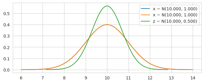
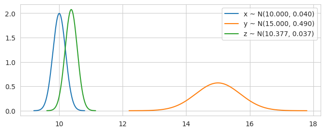
# Product of two different Gaussians.
x = time_ut.Gaussian(10, 0.2**2)
y = time_ut.Gaussian(15, 0.7**2)

z = time_ut.gaussian_multiply(x, y)
print("z=", z)

ax = time_ut.plot_gaussian(x, label="x")
time_ut.plot_gaussian(y, ax=ax, label="y")
_ = time_ut.plot_gaussian(z, ax=ax, label="z")
N(mu=10.377, sigma^2=0.037)
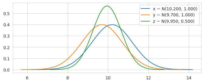
x = time_ut.Gaussian(10.2, 1)
y = time_ut.Gaussian(9.7, 1)

z = time_ut.gaussian_multiply(x, y)
print("z=", z)

ax = time_ut.plot_gaussian(x, label="x")
time_ut.plot_gaussian(y, ax=ax, label="y")
_ = time_ut.plot_gaussian(z, ax=ax, label="z")
N(mu=9.950, sigma^2=0.500)
Implementation: time_ut.cell1_2_plot_gaussian_product()
- Plots input Gaussians (blue) and (yellow) as filled PDFs, the analytical product (red line), and a numerical product via importance sampling (light coral histogram)
hintros.print_obj_info(time_ut.cell1_2_plot_gaussian_product)time_ut.cell1_2_plot_gaussian_product()Usage
Inputs
mu1(): mean ofsigma1(): standard deviation ofmu2(): mean ofsigma2(): standard deviation of
Panels
left: and as filled PDFs, the analytical product , and the sampled numerical product
Guided usage
- Set
sigma1much smaller thansigma2- Observe ’s mean sits close to
mu1: the product pulls the mean toward the more certain (narrower) Gaussian
- Observe ’s mean sits close to
- Set
mu1close tomu2, both with small sigmas- Observe becomes very sharp: when the inputs agree, the product is highly certain
- Compare ’s width to both inputs
- Observe it is always narrower than either input
Part 2: Tracking the Dog
Cell 2.1: The predict-update cycle
- The intuition is the same as the discrete case
- There is a cycle of prediction and updates
- Predict: prior = x_est using system model
- Update: posterior = likelihood * prior
- Create prior (using current estimate and system model)
prior = predict(x, process_model)
- Create likelihood (using measurement)
likelihood = gaussian(z, sensor_var)
- Update belief using prior and likelihood
x = update(prior, likelihood)
- Sum adds uncertainty; multiplication reduces uncertainty
- Let’s assume that the dog moves in the hallway, back and forth (it’s not circular), and we have a sensor that measures the distance of the dog from one extreme
We can use Newton’s equation of motion to compute the position of the dog, based on current position and velocity
- has uncertainty quantified by a Gaussian
- has also uncertainty quantified by a Gaussian
We can compute the sum of 2 Gaussians in terms of mean and uncertainty. It makes sense since we know that uncertainty becomes larger.
The likelihood is the probability of measures given the current state.
Cell 2.2: Simulating the dog and its sensor
Goal:
- Simulate a dog moving at constant velocity, with a noisy sensor, to generate the data the filter will track in Cell 2.3
Implementation: time_ut.DogSimulation(...)
np.random.seed(13)

# Variance in the dog's movement.
process_var = 1.0
# Variance in the sensor.
sensor_var = 2.0

# Dog's initial position.
x = time_ut.Gaussian(0.0, 20.0**2)
velocity = 1.0
# Time step in seconds.
dt = 1.0
# Displacement to add to x (representing how to model the movement of the
# dog).
process_model = time_ut.Gaussian(velocity * dt, process_var)

# Simulate dog and get measurements.
dog = time_ut.DogSimulation(
    x0=x.mean,
    velocity=process_model.mean,
    measurement_var=sensor_var,
    process_var=process_model.var,
)

# Simulate dog and collect measurements and actual positions.
n_steps = 10
sim_data = [dog.move_and_sense() for _ in range(n_steps)]
zs = [m for m, _ in sim_data]
actual_positions = [pos for _, pos in sim_data]
print("zs=", zs)
[1.3535959735108178, 1.8820653967131618, 4.341047429453569, 7.156332673205118, 6.938695089418526, 6.843912342028484, 9.846824080052299, 12.553482049375292, 16.2730841073834, 14.800411177015299]
Cell 2.3: Running the Kalman filter
Goal:
- Run the predict-update cycle from Cell 2.1 on the simulated data, and check that the posterior’s uncertainty settles below the sensor’s
# Perform Kalman filter on measurements.
kf_info = []
for z, actual_pos in zip(zs, actual_positions):
    prior = time_ut.predict(x, process_model)
    likelihood = time_ut.Gaussian(z, sensor_var)
    x = time_ut.update(prior, likelihood)
    kf_info.append(
        time_ut.KfInfo(
            prior=prior, measurement=z, actual_pos=actual_pos, posterior=x
        )
    )

print(time_ut.kf_info_to_df(kf_info))
predict_x predict_var z actual_pos update_x update_var
0 1.000000 401.000000 1.353596 0.287609 1.351841 1.990074
1 2.351841 2.990074 1.882065 1.243106 2.070349 1.198409
2 3.070349 2.198409 4.341047 3.588208 3.735724 1.047258
3 4.735724 2.047258 7.156333 5.938396 5.960160 1.011677
4 6.960160 2.011677 6.938695 8.417082 6.949397 1.002911
5 7.949397 2.002911 6.843912 8.628093 7.396253 1.000727
6 8.396253 2.000727 9.846824 10.190939 9.121670 1.000182
7 10.121670 2.000182 12.553482 12.104680 11.337631 1.000045
8 12.337631 2.000045 16.273084 13.231983 14.305380 1.000011
9 15.305380 2.000011 14.800411 14.838272 15.052895 1.000003
- The uncertainty after prediction is larger than the uncertainty after update (as usual)
- The variance of the prior at time 0 is very large, but after we measure, the variance of the measurement “dominates”
- The posterior values are always between the measurement and the prior
- After a few cycles the posterior variance is around 1, which is smaller than the sensor variance (~2): using a model + measurements is better
# Plot Kalman filter results.
time_ut.plot_kf_info(kf_info, show_actual_pos="scatter")
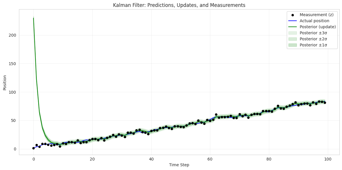
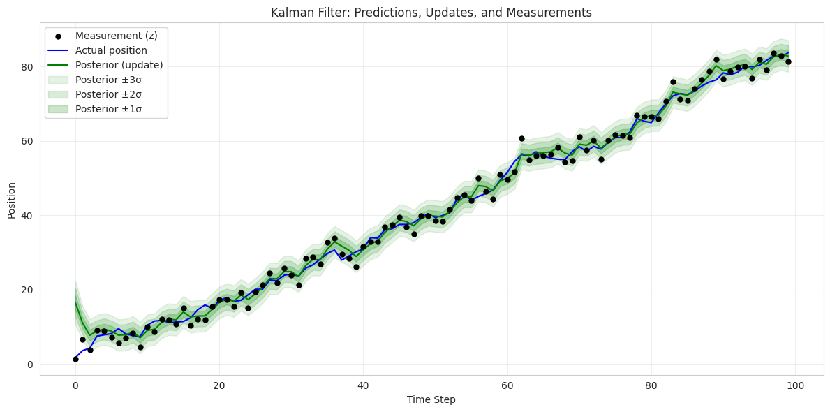
Cell 2.4: Bad initial estimate
Goal:
- Start the filter’s belief far from the dog’s true starting position, and check that it still converges given enough measurements
seed = 42
process_var = 2.0
sensor_var = 2.0**2
# Belief about initial position.
initial_position = 400
initial_pos_var = 1.0
# Actual initial position.
actual_initial_pos = 0.0
n_steps = 100

kf_info = time_ut._run_dog_simulation(
    seed,
    process_var,
    sensor_var,
    initial_position,
    actual_initial_pos=actual_initial_pos,
    initial_pos_var=initial_pos_var,
    n_steps=n_steps,
)
time_ut.plot_kf_info(
    kf_info, show_prior="none", show_actual_pos="line", show_posterior="line"
)
# Belief about initial position.
initial_position = 400
initial_pos_var = 100.0
# Actual initial position.
actual_initial_pos = 0.0

kf_info = time_ut._run_dog_simulation(
    seed,
    process_var,
    sensor_var,
    initial_position,
    actual_initial_pos=actual_initial_pos,
    initial_pos_var=initial_pos_var,
    n_steps=n_steps,
)
time_ut.plot_kf_info(
    kf_info, show_prior="none", show_actual_pos="line", show_posterior="line"
)
Cell 2.5: Extreme amount of noise
Goal:
- Push the sensor noise to an extreme, and check that the filter still recovers the dog’s position as long as the process model is trusted
seed = 42
process_var = 2.0
sensor_var = 300.0**2
initial_position = 0.0
n_steps = 1000

kf_info = time_ut._run_dog_simulation(
    seed, process_var, sensor_var, initial_position, n_steps=n_steps
)
time_ut.plot_kf_info(
    kf_info, show_prior="none", show_actual_pos="line", show_posterior="line"
)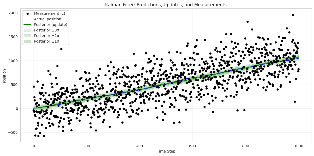
- Even with extreme amounts of noise we recover the position of the dog
- This is because the process error is small (we can trust the model)
Cell 2.6: Too much belief in the model
Goal:
- Have the dog accelerate, violating the constant-velocity process model, and check that an over-confident filter fails to track it
seed = 42
process_var = 2.0
sensor_var = 300.0**2
acceleration = 0.04
initial_position = 0.0
n_steps = 300

kf_info = time_ut._run_dog_simulation(
    seed,
    process_var,
    sensor_var,
    initial_position,
    acceleration=acceleration,
    n_steps=n_steps,
)
time_ut.plot_kf_info(
    kf_info, show_prior="none", show_actual_pos="line", show_posterior="line"
)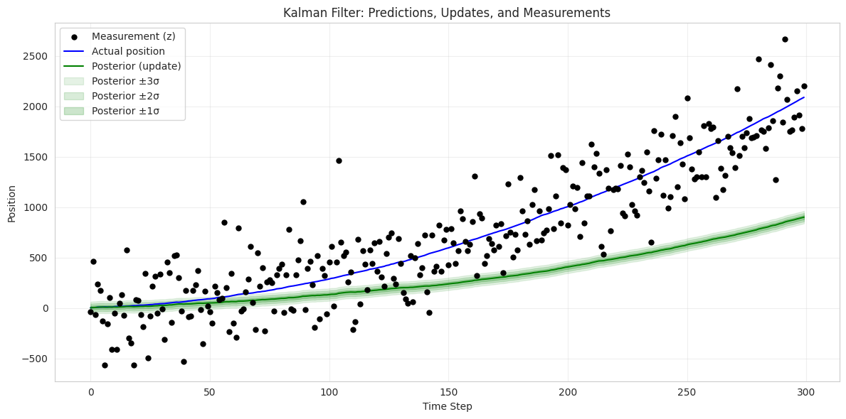
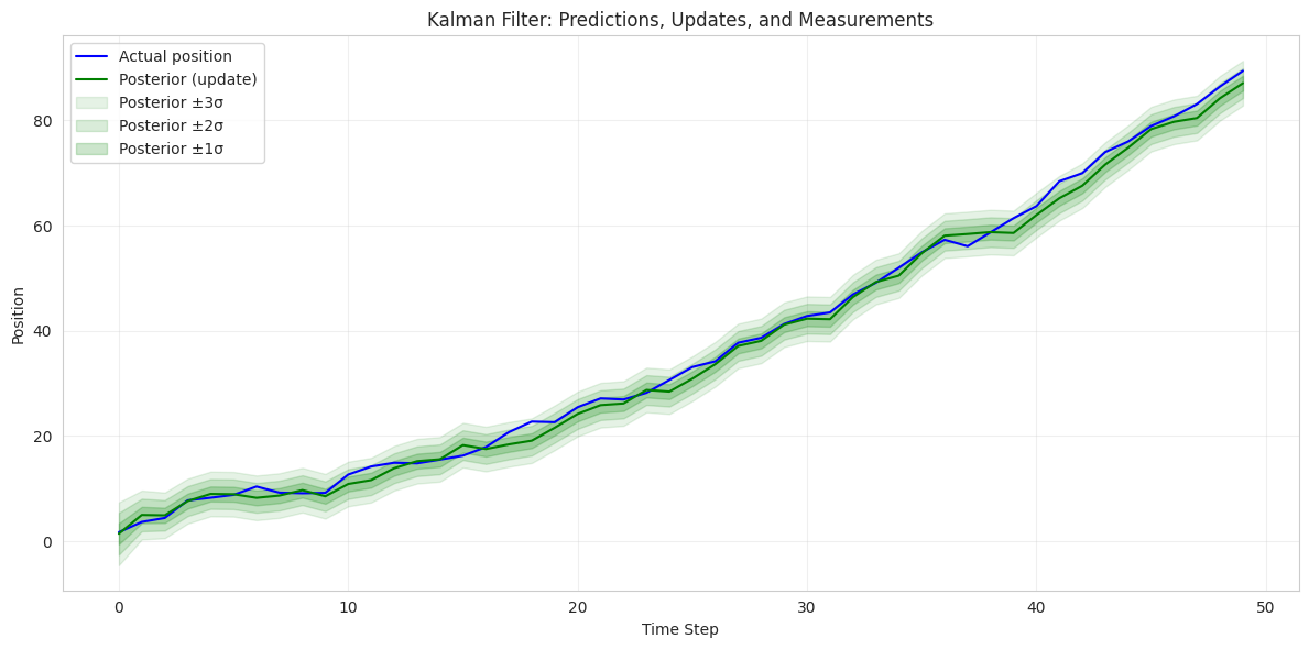
- The filter is not able to follow the change of velocity of the dog
seed = 42
process_var = 2.0
sensor_var = 2.0**2
acceleration = 0.04
initial_position = 0.0
n_steps = 50

kf_info = time_ut._run_dog_simulation(
    seed,
    process_var,
    sensor_var,
    initial_position,
    acceleration=acceleration,
    n_steps=n_steps,
)
time_ut.plot_kf_info(
    kf_info,
    show_prior="none",
    show_actual_pos="line",
    show_posterior="line",
    show_measurements="none",
)
Cell 2.7: Interactively exploring the filter
Goal:
- Let students sweep every parameter from Cells 2.4-2.6 at once, to consolidate the intuition for how the filter balances the process model against sensor measurements
Implementation: time_ut.cell2_interactive_dog_simulation()
- Prior (predict) as red up-triangles: prediction from motion model
- Measurement as black circles: noisy sensor readings
- Posterior (update) as green down-triangles: filtered estimate
- Posterior uncertainty as shaded green bands (+-1, 2, 3 sigma)
hintros.print_obj_info(time_ut.cell2_interactive_dog_simulation)time_ut.cell2_interactive_dog_simulation()Usage
Inputs
process_var(): variance in the dog’s movement modelsensor_var(): variance in the sensor measurementsinitial_position(): belief about the dog’s starting positionactual_initial_pos: the dog’s true starting position (can differ from the belief to simulate a wrong initial estimate)initial_pos_var: uncertainty (variance) in the initial position belief; large values mean we are very uncertain about where the dog startsacceleration: dog’s acceleration (); non-zero values make the dog speed up over time, testing the filter’s ability to trackseed: random seed for reproducibility
Panels
left: prior, measurements, posterior, and posterior uncertainty bands over timeComments: the current parameters, and the final posterior mean/variance
Guided usage
- Lower
sensor_varfar belowprocess_var- Observe the posterior in Comments tracks the measurements closely: the filter trusts the sensor
- Lower
process_varfar belowsensor_var- Observe the posterior changes less: the motion model dominates
- Let the simulation run its full 25 steps
- Observe the final posterior variance in Comments stabilizes below both input variances
- Is it better to have precise measurements (
sensor_var<<process_var) or vice versa?