Non-linear Kalman filter - MSML610 -- Tutorials

Imports¶

%load_ext autoreload
%autoreload 2

import logging

import numpy as np
from numpy.random import multivariate_normal, normal

import helpers.htutorial as ut

ut.config_notebook()

# Initialize logger.
logging.basicConfig(level=logging.INFO)
_LOG = logging.getLogger(__name__)

WARNING (pytensor.tensor.blas): Using NumPy C-API based implementation for BLAS functions.
vim support installed: restart the notebook, if needed

Python 3.12.3
Linux b556f3ab449c 6.12.67-linuxkit #1 SMP Sun Jan 25 02:26:28 UTC 2026 aarch64 aarch64 aarch64 GNU/Linux

import helpers.hio as hio
import L09_05_04_non_linear_kalman_filter_utils as time_ut

dst_dir = "figures"
hio.create_dir(dst_dir, incremental=True)
!cp msml610/tutorials/figures/*.png msml610/lectures_source/figures

# `filterpy` is an extra for this notebook, pinned to the version already
# in requirements.txt.
!sudo /bin/bash -c "(source /venv/bin/activate; pip install --quiet filterpy==1.4.5)"

Part 1: Nonlinear Transformations of a Gaussian¶

Cell 1.1: A nonlinear 1D function¶

Goal:

Look at a nonlinear function before checking what it does to a Gaussian input

Implementation: time_ut.plot_function(f)

def f(x):
    return (np.cos(4 * (x / 2 + 0.7))) - 1.3 * x


time_ut.plot_function(f)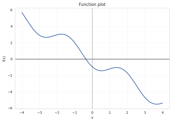

Cell 1.2: How a nonlinear function distorts a Gaussian¶

Goal:

Push a large Gaussian sample through f, to see that the output is no longer Gaussian, and that the naive “linearized” mean $f(\mu)$ diverges from the true mean $E[f(X)]$

Implementation: time_ut.plot_nonlinear_func(data, f)

# Create 500,000 samples with mean 0, std 1.
gaussian = (0.0, 1.0)
data = normal(loc=gaussian[0], scale=gaussian[1], size=500000)

time_ut.plot_nonlinear_func(data, f)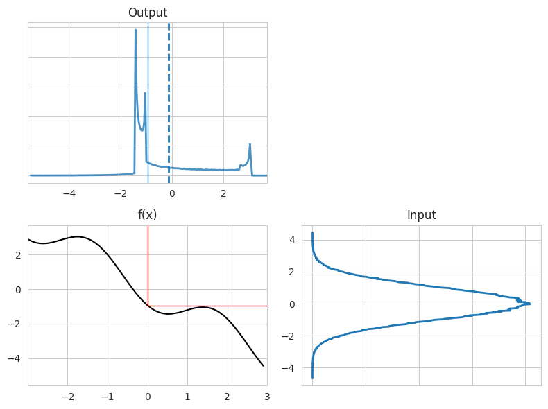

Cell 1.3: Visualizing input vs output samples¶

Goal:

Compare individual input samples against their transformed output, to see how f reshapes the distribution point by point

Implementation: time_ut.plot_input_output_scatter(data, f, n)

# Plot N points.
N = 30000
time_ut.plot_input_output_scatter(data, f, N)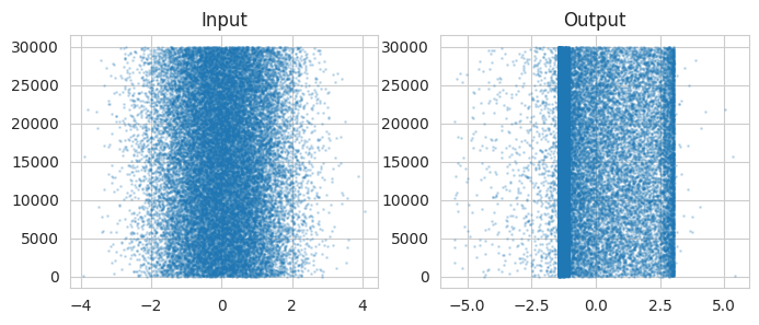

Part 2: Nonlinear Transformations in 2D¶

Cell 2.1: A nonlinear 2D function¶

Goal:

Look at a 2D nonlinear function, mapping a plane into a (sum, weighted-sum-of-squares) space, as the running example for the rest of this notebook

Implementation: time_ut.plot_nonlinear_xy()

def f_nonlinear_xy(x, y):
    return np.array([x + y, 0.1 * x**2 + y * y])


time_ut.plot_nonlinear_xy()

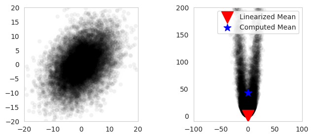
Cell 2.2: Linearized mean vs Monte Carlo mean¶

Goal:

Compare 2 ways of estimating $E[f(X, Y)]$ for a 2D Gaussian input: plugging the input mean into f (linearized mean, cheap but biased for a nonlinear f), vs averaging f over many samples (Monte Carlo mean, accurate but expensive)

Implementation: time_ut.plot_monte_carlo_mean(...)

# Create a Gaussian.
N = 10000
mean = (0.0, 0.0)
p = np.array([[32.0, 15.0], [15.0, 40.0]])
xs, ys = multivariate_normal(mean=mean, cov=p, size=N).T

# Compute linearized mean.
mean1 = f_nonlinear_xy(np.mean(xs), np.mean(ys))
_LOG.info("f(mean)=%s", mean1)
mean2 = np.mean(
    [f_nonlinear_xy(xs_tmp, ys_tmp) for xs_tmp, ys_tmp in zip(xs, ys)], axis=0
)
_LOG.info("mean(f)=%s", mean2)
# Plot both.
time_ut.plot_monte_carlo_mean(xs, ys, f_nonlinear_xy, mean1, "Linearized Mean")

INFO:__main__:f(mean)=[0.06708904 0.00185213]
INFO:__main__:mean(f)=[ 0.06708904 43.25045478]

Part 3: The Unscented Transform¶

Cell 3.1: Generating sigma points¶

Goal:

Replace the full Monte Carlo sample with a small, deterministic set of “sigma points” that captures the same mean and covariance

Implementation: filterpy.kalman.MerweScaledSigmaPoints(...), time_ut.plot_sigma_points(mean, p, sigmas)

from filterpy.kalman import MerweScaledSigmaPoints

# Initial mean and covariance.
mean = (0.0, 0.0)
p = np.array([[32.0, 15.0], [15.0, 40.0]])

# Create sigma points and weights from the initial distribution.
points = MerweScaledSigmaPoints(n=2, alpha=0.3, beta=2.0, kappa=0.1)
sigmas = points.sigma_points(mean, p)

time_ut.plot_sigma_points(mean, p, sigmas)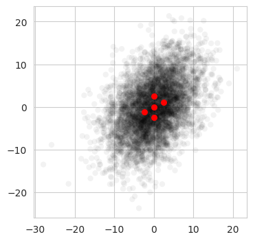

Cell 3.2: Propagating sigma points through the nonlinear function¶

Goal:

Push only the 5 sigma points through f_nonlinear_xy, then recombine them (the “unscented transform”) into a new mean and covariance, and compare against the Monte Carlo mean from Cell 2.2

Implementation: filterpy.kalman.unscented_transform(...), time_ut.plot_monte_carlo_mean(...)

from filterpy.kalman import unscented_transform

# Transform sigma points through non-linear function.
sigmas_f = np.empty((5, 2))
for i in range(5):
    sigmas_f[i] = f_nonlinear_xy(sigmas[i, 0], sigmas[i, 1])

# Use unscented transform to get new mean and covariance.
ukf_mean, ukf_cov = unscented_transform(sigmas_f, points.Wm, points.Wc)

# Generate random points.
np.random.seed(100)
xs, ys = multivariate_normal(mean=mean, cov=p, size=5000).T
time_ut.plot_monte_carlo_mean(xs, ys, f_nonlinear_xy, ukf_mean, "Unscented Mean")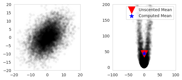

Using only 5 points we were able to compute the mean with great accuracy

Cell 3.3: Comparing the linearized and unscented means¶

Goal:

Compare the cheap-but-biased linearized mean against the 5-point unscented mean, side by side

# Compute linearized mean.
mean1 = f_nonlinear_xy(np.mean(xs), np.mean(ys))
_LOG.info("f(mean)=%s", mean1)
_LOG.info("mean(f)=%s", ukf_mean)

INFO:__main__:f(mean)=[-0.0965117   0.00646045]
INFO:__main__:mean(f)=[2.00589856e-15 4.32000000e+01]