Imports
%load_ext autoreload
%autoreload 2

import logging

import matplotlib.pyplot as plt
import numpy as np

import helpers.hintrospection as hintros
import helpers.htutorial as ut

ut.config_notebook()

# Initialize logger.
logging.basicConfig(level=logging.INFO)
_LOG = logging.getLogger(__name__)
The autoreload extension is already loaded. To reload it, use:
%reload_ext autoreload
WARNING:msml610_utils:vim support installed: restart the notebook, if needed
INFO:msml610_utils:Setting notebook style
INFO:msml610_utils:Notebook signature
INFO:msml610_utils:numpy version=1.26.4
INFO:msml610_utils:pymc version=5.18.2
INFO:msml610_utils:matplotlib version=3.10.3
INFO:msml610_utils:arviz version=0.21.0
INFO:msml610_utils:preliz version=0.19.0
Python 3.12.3
Linux 7d77d2247121 6.12.67-linuxkit #1 SMP Sun Jan 25 02:26:28 UTC 2026 aarch64 aarch64 aarch64 GNU/Linux
import helpers.hio as hio
import L09_05_03_multivariate_kalman_filter_utils as time_ut

dst_dir = "figures"
hio.create_dir(dst_dir, incremental=True)
!cp msml610/tutorials/figures/*.png msml610/lectures_source/figures
# `filterpy` is an extra for this notebook, pinned to the version already
# in requirements.txt.
!sudo /bin/bash -c "(source /venv/bin/activate; pip install --quiet filterpy==1.4.5)"
import filterpyPart 1: Multivariate Gaussians
Cell 1.1: Correlated variables and covariance
- A multivariate Gaussian is a normal distribution on multiple
dimensions
- The dimensions don’t need to be necessarily spatial dimensions
- E.g., position, velocity, acceleration in 3 dimensions
- E.g., milk production and feed rate at a dairy
- The components of a Gaussian are correlated
- E.g., height and weight of people are (positively) correlated
- E.g., outdoor temperature and home heating bills are (negatively) correlated
- E.g., the weight of my dog and the price of coffee are uncorrelated
- Correlation allows prediction
- E.g., height and weight are correlated. If you are much taller than me, I can predict that you weigh more than me
- Noise in the measurements, uncertainty in the knowledge of the system, intrinsic stochasticity make correlations (and predictions) imperfect
- Assuming linear correlation, the covariance between 2 vars is defined as
height = [60, 62, 63, 65, 65.1, 68, 69, 70, 72, 74]
weight = [95, 120, 127, 119, 151, 143, 173, 171, 180, 210]
time_ut.plot_correlated_data(
    height, weight, xlabel="Height (in)", ylabel="Weight (lbs)", equal=False
)
print("cov=\n", np.cov(height, weight))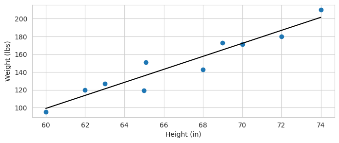
cov=
 [[  20.58322222  150.77888889]
 [ 150.77888889 1213.65555556]]
Cell 1.2: The multivariate Gaussian PDF
Goal:
- Evaluate the multivariate Gaussian PDF at a point, given a mean vector and a covariance matrix
Implementation: filterpy.stats.multivariate_gaussian(x, mu, P)
from filterpy.stats import multivariate_gaussian

x = np.array([2.5, 7.3])
mu = np.array([2.0, 7.0])
P = np.array([[8.0, 0.0], [0.0, 3.0]])

print("multivariate_gaussian=", multivariate_gaussian(x, mu, P))0.031507521572225645Cell 1.3: Visualizing a 2D covariance
Goal:
- Visualize a 2D Gaussian’s covariance both as a 3D sampled surface and as a 2D covariance-ellipse-style matrix plot
Implementation: time_ut.plot_3d_sampled_covariance(mu, P),
time_ut.cell_1_1_plot_covariance_matrix()
time_ut.plot_3d_sampled_covariance(mu, P)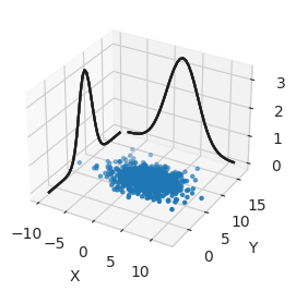
hintros.print_obj_info(time_ut.cell_1_1_plot_covariance_matrix)time_ut.cell_1_1_plot_covariance_matrix()Usage
Inputs
sigma_x,sigma_y: standard deviations along each axisrho: correlation coefficient between the 2 axes
Panels
left: the resulting covariance matrix as a heatmapright: the corresponding covariance ellipse
Guided usage
- Set
rho=0, withsigma_x != sigma_y- Observe the ellipse is axis-aligned
- Raise
rhotoward1- Observe the ellipse tilts and elongates along the diagonal
Cell 1.4: Using correlations to improve estimates
- Given an aircraft that we need to locate on a 2D map, ignoring the altitude
- We are tracking an aircraft with 2 radars
- Each radar provides the position as 2 coordinates, such as the “range” (distance) and the “bearing” (angle) to a target
- The areas on the X-Y diagrams represent where the plane is likely to be
- One radar measurement (let’s assume it’s the prior) is equally distributed across the 2 axes (yellow)
- The other radar measurement (let’s assume it’s the evidence) instead is inaccurate along the range but precise along the bearing estimates (green)
- The posterior is given by the multiplication of the 2 Gaussians (blue): its uncertainty is smaller than either of the 2 measurements
# Prior.
P0 = [[6, 0], [0, 6]]
filterpy.stats.plot_covariance_ellipse((10, 10), P0, fc="y", alpha=0.6)

# Evidence.
P1 = [[2, 1.9], [1.9, 2]]
filterpy.stats.plot_covariance_ellipse((10, 10), P1, fc="g", alpha=0.9)

# Posterior.
P2 = filterpy.stats.multivariate_multiply((10, 10), P0, (10, 10), P1)[1]
print("P2=", P2)
filterpy.stats.plot_covariance_ellipse((10, 10), P2, ec="k", fc="b")
[[1.23099851 1.13263785]
[1.13263785 1.23099851]]
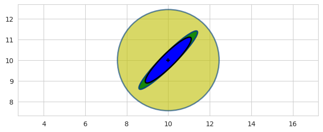
- If the 2 measurements are like below, the resulting measurement is
much smaller
- We are “triangulating” the aircraft
- This is optimal when the radars are orthogonal
P3 = [[2, -1.9], [-1.9, 2.2]]
filterpy.stats.plot_covariance_ellipse((10, 10), P2, ec="k", fc="y", alpha=0.6)
filterpy.stats.plot_covariance_ellipse((10, 10), P3, ec="k", fc="g", alpha=0.6)

P4 = filterpy.stats.multivariate_multiply((10, 10), P2, (10, 10), P3)[1]
filterpy.stats.plot_covariance_ellipse((10, 10), P4, ec="k", fc="b")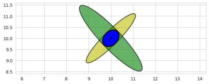
Part 2: Sum and Product of Bidimensional Gaussians
Cell 2.1: Sum of 2 2D Gaussians
- If and are
independent, then : the
covariances add
- Yellow: G1
- Green: G2
- Blue: G1 + G2
- The sum is always larger (less certain) than either factor
Implementation: time_ut.cell_1_2_plot_sum_of_gaussians()
time_ut.cell_1_2_plot_sum_of_gaussians()Cell 2.2: Product of 2 2D Gaussians
- The product of 2 Gaussian PDFs is also a Gaussian (up to normalization)
- Given and :
- Yellow: G1
- Green: G2
- Blue: G1 * G2
- The product is always smaller (more certain) than either factor
Implementation: time_ut.cell_1_3_plot_product_of_gaussians()
time_ut.cell_1_3_plot_product_of_gaussians()Part 3: Tracking a Dog with Hidden Variables
- We go back to tracking a dog on a 1D track and use hidden variables
to improve our estimates
- The underlying ideas are the same as the previous chapters: we are just multiplying and adding Gaussians
- The dog moves approximately 1 meter per step
- At each step, the velocity varies according to the process
variance
process_var - After updating the position, a measurement is computed with an
assumed sensor variance
z_var - Time is discrete
- At each step, the velocity varies according to the process
variance
Cell 3.1: Simulating the dog
Goal:
- Simulate the dog’s true trajectory and noisy sensor measurements, used throughout the rest of Part 3
Implementation: time_ut.compute_dog_data(z_var, process_var, count)
z_var = 1.0
process_var = 0.1
count = 50
xs, zs = time_ut.compute_dog_data(z_var, process_var, count=count)
print("xs=", xs)
print("zs=", zs)
xs= [ 0.65477387 1.87472222 2.78176171 3.30176789 4.58333177 5.74165617
6.74388974 7.96487869 9.12046871 9.43952189 10.28810019 11.50739747
12.84257879 14.05874239 15.44199273 16.32521704 16.76352214 17.43800629
17.95659405 18.75760349 19.58816819 20.23509216 21.18579283 22.23639503
23.58974756 24.47597873 25.34522957 26.04046223 27.14917751 28.15954883
29.08668972 30.36819518 30.78437932 31.31113521 32.28474981 32.99323214
34.05877583 34.83054237 35.65766695 37.18685897 37.77589529 39.03248141
40.29140164 40.9364218 42.25823461 43.43262673 44.55617562 45.88736656
46.81482684 47.33064813]
zs= [ 0.26767417 2.72382433 2.71016246 2.94473869 5.15853678 5.79142986
6.0835686 8.38585163 8.59443386 10.5366746 9.42532442 11.11538483
13.45958474 12.69278668 15.70324326 16.46860551 17.17217495 16.085336
19.06928242 20.2913312 17.88081023 21.47090378 20.63750553 22.73817777
25.03824679 23.14993104 25.60551007 25.08331132 27.10052516 27.40105349
28.16245658 31.40344451 29.85486846 30.66111128 30.83510459 31.98927477
34.12812016 35.00736324 35.38601184 38.52732002 38.60562771 37.88421812
41.82933356 40.01891898 42.52972993 43.77321594 43.2297035 47.05695655
46.77134989 47.84490289]
plt.figure(figsize=(8, 3))
_ = plt.plot(xs, label="True position (xs)")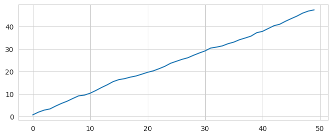
Cell 3.2: Predict step: the state vector
- The state vector tracks both position and velocity:
- Position is observed by the sensor
- Velocity is a hidden variable: it is estimated by the filter, not measured directly
- Additional hidden variables (e.g., acceleration, jerk) can be added at the cost of a larger state vector
dt = 1.0  # Time step (seconds).
# Initial state: position 0 m, velocity 1 m/s.
x0 = np.array([[0.0], [1.0]])
print("x0 (initial state) =\n", x0)
x0 (initial state) =
[[0.]
[1.]]
Cell 3.3: Designing the state covariance
- The state covariance matrix encodes our uncertainty about the state
- We initialize it with large diagonal values to reflect ignorance at
startup:
- : we do not know the dog’s starting position
- : top dog speed is 21 m/s, so
- Off-diagonal terms are zero: position and velocity are initially uncorrelated
# Initial state covariance: large uncertainty in position and velocity.
P = np.diag([500.0, 49.0])
print("P =\n", P)
Cell 3.4: Designing the system model
- The state-transition matrix describes how the state evolves over one time step under a constant-velocity assumption:
- In matrix form :
- The constant-velocity assumption is approximate; the filter tolerates deviations through the process noise
# State transition matrix: constant velocity model.
F = np.array([[1.0, dt], [0.0, 1.0]])
print("F =\n", F)
F =
[[1. 1.]
[0. 1.]]
Cell 3.5: Predicting the system
- Without a new measurement the filter propagates the state and covariance forward (the predict step):
- The covariance grows at every prediction step because the future velocity is uncertain; adding measurements (update step) shrinks it back
# One illustrative prediction step (no measurement yet, Q = 0 for clarity).
x_pred = F @ x0
P_pred = F @ P @ F.T
print("x_pred (one step) =\n", x_pred)
print("P_pred (one step) =\n", P_pred)
x_pred (one step) =
[[1.]
[1.]]
P_pred (one step) =
[[549. 49.]
[ 49. 49.]]
Cell 3.6: Designing the system noise
- The dog’s velocity is not perfectly constant; it is perturbed by unmodeled forces (distraction, fatigue, wind)
- We model the velocity perturbation as zero-mean Gaussian noise :
- The process noise covariance captures this uncertainty
- Position is not directly noisy (it inherits noise only through velocity), so only the velocity variance is non-zero:
# Process noise covariance: only velocity is directly perturbed.
Q = np.array([[0.0, 0.0], [0.0, process_var]])
print("Q =\n", Q)
Q =
[[0. 0. ]
[0. 0.1]]
Cell 3.7: Designing the control function
- A known control input can shift the predicted state:
- Examples of control inputs:
- Car: steering angle, throttle
- Dog: the owner’s voice command, the sight of a squirrel
- In this example there is no known control input, so
# No control input in this example.
B = np.zeros((2, 1))
u = np.zeros((1, 1))
print("B =\n", B)
print("u =\n", u)
B =
[[0.]
[0.]]
u =
[[0.]]
Cell 3.8: Update step: the measurement function
- The sensor measures only position, not velocity
- The measurement is related to the full state via the measurement matrix :
- For position-only observation:
- The innovation (residual) is the difference between the actual measurement and the predicted measurement:
# Measurement matrix: H selects position from the state vector.
H = np.array([[1.0, 0.0]])
print("H =", H)
Cell 3.9: Designing the measurement noise matrix R
- encodes the variance of the sensor noise:
- can be difficult to estimate in practice:
- Noise may not be Gaussian
- There can be a systematic bias in the sensor
- The error can be asymmetric (e.g., a temperature sensor is less precise at high temperatures)
# Measurement noise covariance.
R = np.array([[z_var]])
print("R =", R)
R = [[1.]]
Cell 3.10: Running the Kalman filter
Goal:
- Run the full predict-update cycle on the simulated dog data, and check that the estimate converges close to the true position
Implementation: time_ut.run_dog_kalman_filter(zs, z_var, process_var)
- The filter alternates predict and update at every time step
- After a few steps the estimate converges close to the true position
- The uncertainty (shaded band) shrinks rapidly as measurements accumulate
means, variances = time_ut.run_dog_kalman_filter(zs, z_var, process_var)
time_ut.plot_dog_tracking(xs, zs, means, variances)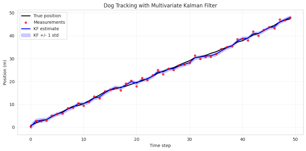
Cell 3.11: Interactively exploring dog tracking
Goal:
- Let students sweep the noise levels and see the filter adapt in real time
Implementation: time_ut.cell_dog_tracking_interactive()
- Increasing
z_varmakes the sensor noisier: the filter smooths more aggressively and leans on its own prediction - Increasing
process_varmakes the dog more unpredictable: the filter trusts measurements more and follows them closely - The blue band shows the +-1 sigma position uncertainty of the filter
hintros.print_obj_info(time_ut.cell_dog_tracking_interactive)time_ut.cell_dog_tracking_interactive()Usage
Inputs
seed: random seed for reproducibilityz_var: measurement noise varianceprocess_var: process noise variancecount: number of simulation steps
Panels
left: true position, measurements, KF estimate, and +-1 std dev bandComments: the current parameters, and the final estimate’s MSE against the true position
Guided usage
- Raise
z_varfar aboveprocess_var- Observe the KF estimate line smooths out, tracking its own prediction more than the noisy measurements
- Raise
process_varfar abovez_var- Observe the KF estimate follows the measurements closely
Part 4: Effect of Hidden Variables
Cell 4.1: What changes when we add a hidden variable?
- A 1D Kalman filter tracks position only:
- The filter has no model of velocity; it assumes the dog is stationary between measurements
- Each prediction step simply holds position constant:
- The filter can only react to measurements, not anticipate movement
- A 2D Kalman filter tracks position and velocity:
- Velocity is the hidden variable: never measured directly, but inferred from successive position measurements
- The prediction step uses velocity to anticipate where the dog will be:
- The covariance matrix develops off-diagonal terms that capture the correlation between position and velocity errors
Why hidden variables help
- The 1D filter is essentially a recursive average: it is well-calibrated only when the dog is stationary or very slow
- The 2D filter learns the dog’s speed implicitly; after a few steps the estimated velocity is close to the true velocity and the position predictions are much more accurate
- The improvement is quantified by the Mean Squared Error (MSE) shown below: the 2D filter consistently achieves a lower MSE than the 1D filter
Experiment setup
- Same dog simulation: the dog moves ~1 m/step with Gaussian velocity noise
- Same measurements: position + Gaussian sensor noise
- 1D filter: , , ,
- 2D filter: , , ,
Implementation: time_ut.plot_hidden_variable_comparison(...)
# Static comparison with default parameters.
np.random.seed(42)
xs_ex, zs_ex = time_ut.compute_dog_data(z_var=1.0, process_var=0.1, count=50)
means_1d, var_1d = time_ut.run_dog_kalman_filter_1d(
    zs_ex, z_var=1.0, process_var=0.1
)
means_2d, var_2d = time_ut.run_dog_kalman_filter(
    zs_ex, z_var=1.0, process_var=0.1
)
time_ut.plot_hidden_variable_comparison(
    xs_ex, zs_ex, means_1d, var_1d, means_2d, var_2d
)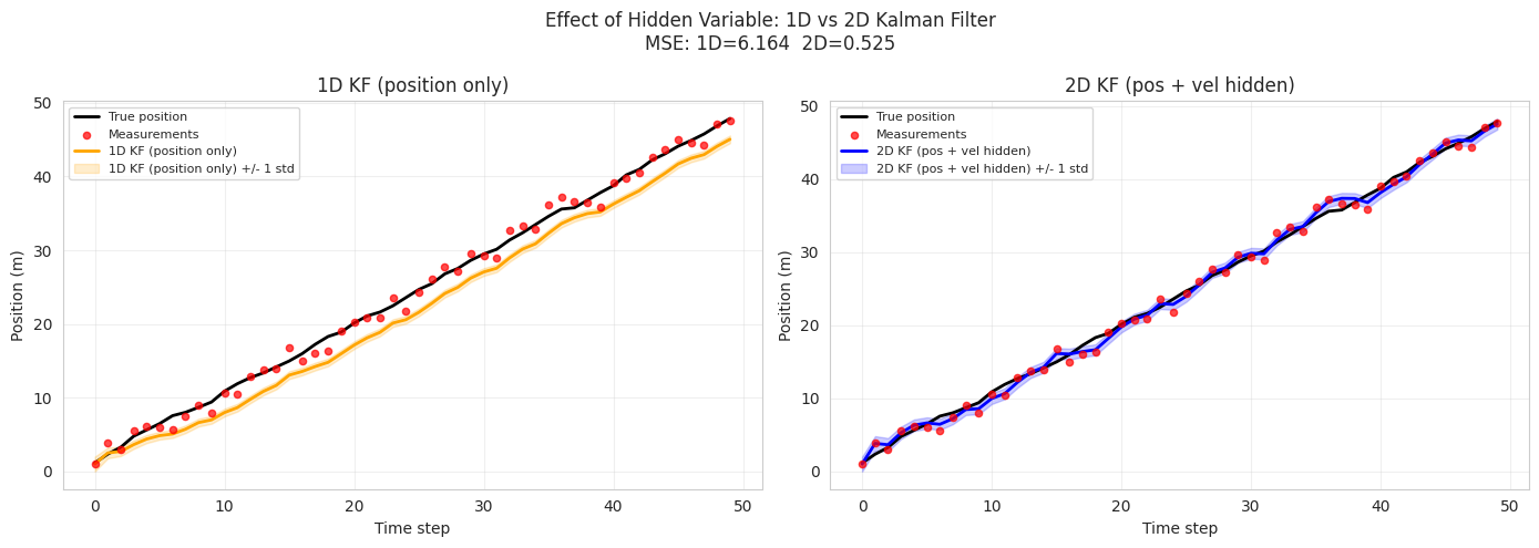
- Left panel (1D KF, position only):
- The filter lags behind the true trajectory because each prediction step does not use velocity: it simply holds the previous position estimate
- The uncertainty band (shaded area) is wide because the filter must account for large unpredicted jumps in position
- MSE is typically higher
- Right panel (2D KF, position + hidden velocity):
- The filter rapidly learns the dog’s velocity from the first few measurements
- Subsequent predictions are accurate because the motion model () anticipates where the dog will be
- The uncertainty band is narrower and centered on the true trajectory
- MSE is consistently lower
Cell 4.2: Interactively comparing 1D vs 2D filters
Goal:
- Let students vary the noise levels and see the MSE gap between the 1D and 2D filters change in real time
Implementation: time_ut.cell_hidden_variable_comparison_interactive()
- Increasing
z_var: both filters degrade, but the 2D filter degrades less because it uses its motion model to bridge noisy measurements - Increasing
process_var: the dog’s velocity changes more erratically; the advantage of the 2D filter is reduced but still present
hintros.print_obj_info(time_ut.cell_hidden_variable_comparison_interactive)time_ut.cell_hidden_variable_comparison_interactive()Usage
Inputs
seed: random seed for reproducibilityz_var: measurement noise varianceprocess_var: process noise variancecount: number of simulation steps
Panels
left: 1D filter (position only) trackingmiddle: 2D filter (position + hidden velocity) trackingComments: the current parameters, both filters’ MSE, and which one wins
Guided usage
- Raise
process_varwhile keepingz_varlow- Observe the MSE gap between the 2 filters in Comments narrows: the 2D filter’s advantage shrinks when the dog’s own motion is erratic
- Raise
z_varwhile keepingprocess_varlow- Observe both MSEs grow, but the 2D filter’s MSE stays lower: it still benefits from anticipating motion even with noisy sensors