Imports
%load_ext autoreload
%autoreload 2

import arviz as az
import pymc as pm
import numpy as np
import scipy.stats as stats
import matplotlib.pyplot as plt
import preliz as pz
from IPython.display import display
import helpers.hintrospection as hintros
import helpers.htutorial as ut
import L07_01_bayesian_coin_utils as coin_ut
ut.config_notebook()Part 1: Probability Distributions
Cell 1.1: Bernoulli
Goal:
- Build intuition for the Bernoulli distribution, a single trial with two outcomes
- means and ,
Implementation: cell1_1_sample_bernoulli_widget()
- Draws
nsamples fromscipy.stats.bernoulli(p)and prints them
hintros.print_obj_info(coin_ut.cell1_1_sample_bernoulli_widget)Usage
Inputs
n: number of samples drawn, 1-50p: success probability, 0-1
Panels
data: printed array ofnrealizations, each 0 or 1
coin_ut.cell1_1_sample_bernoulli_widget()Guided usage
- Raise
pfrom 0 toward 1, leavingnfixed- Observe the printed
datashift from mostly 0s to mostly 1s: a coin flip is if heads, if tails, andpis the heads probability
- Observe the printed
Cell 1.2: Binomial
Goal:
- Build intuition for the binomial distribution, the count of successes
over
trialsindependent Bernoulli draws
Implementation: cell1_2_sample_binomial_widget()
- Draws
nsamples fromscipy.stats.binom(trials, p)and prints them
hintros.print_obj_info(coin_ut.cell1_2_sample_binomial_widget)Usage
Inputs
n: number of samples drawn, 1-50trials: trials per sample, 1-100p: success probability, 0-1
Panels
data: printed array ofnrealizations, each a count in[0, trials]
coin_ut.cell1_2_sample_binomial_widget()Guided usage
- Raise
trialsfrom 1 toward 100, leavingpfixed- Observe the printed counts spread over a wider range: e.g. flipping
a fair coin 10 times, the number of heads follows
Binomial(10, 0.5)
- Observe the printed counts spread over a wider range: e.g. flipping
a fair coin 10 times, the number of heads follows
Cell 1.3: Interactive binomial PMF
Goal:
- Explore the binomial PMF’s shape directly through
preliz’s own interactive widget
Implementation: pz.Binomial(p, n).plot_interactive(**params)
prelizbuilds and displays its own sliders forpandn;kindandintervalcontrol how the distribution is summarized
# Probability of k successes on N trials flipping a coin with p success.
params = {
    # "kind": "cdf",
    "kind": "pdf",
    "pointinterval": False,
    "interval": "hdi",  # Highest density interval.
    # "interval": "eti",  # Equally tailed interval.
    "xy_lim": "auto",
}
pz.Binomial(p=0.5, n=5).plot_interactive(**params)
WARNING (pytensor.tensor.blas): Using NumPy C-API based implementation for BLAS functions.
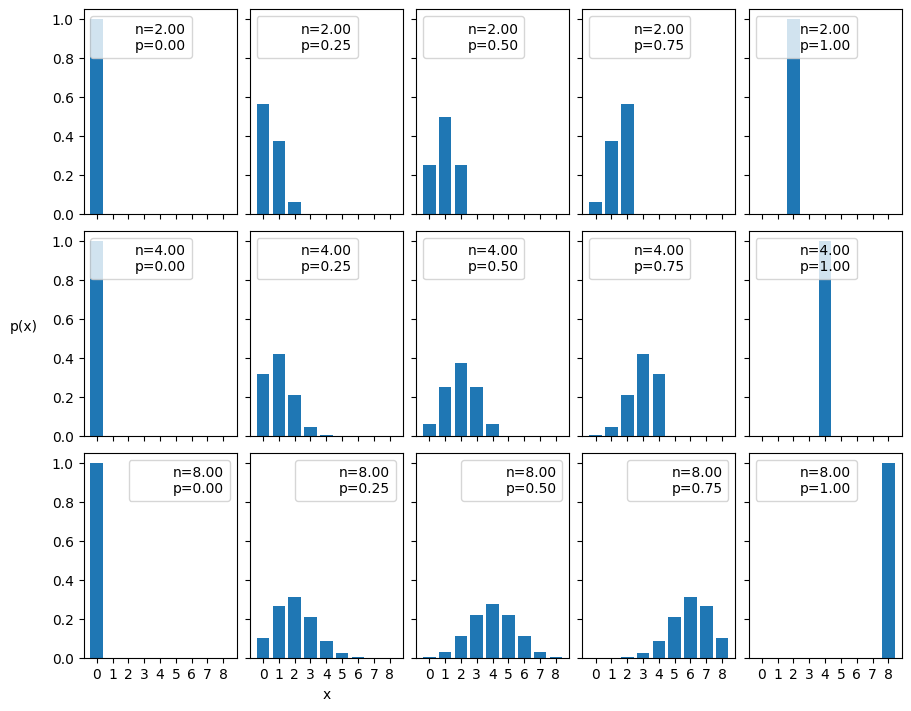
Cell 1.4: Binomial distribution grid
Goal:
- Compare the binomial PMF’s shape across a grid of
nandpvalues at once
Implementation: plot_binomial()
- Plots
stats.binom(n, p).pmf(x)for every combination of 3nvalues and 5pvalues, one subplot each
coin_ut.plot_binomial()(3, 5)
Cell 1.5: Beta
Goal:
- Build intuition for the Beta distribution, a continuous distribution on used to model a probability or proportion
ais the “success” shape parameter,bis the “failure” shape parameter:a>bskews the density toward 1,a=bcenters it on 0.5
Implementation: cell1_5_sample_beta_widget()
- Draws
nsamples fromscipy.stats.beta(a, b)and prints them
hintros.print_obj_info(coin_ut.cell1_5_sample_beta_widget)Usage
Inputs
n: number of samples drawn, 1-50a: alpha shape parameter, 0.1-10b: beta shape parameter, 0.1-10
Panels
data: printed array ofnrealizations in[0, 1]
coin_ut.cell1_5_sample_beta_widget()Guided usage
- Set
awell aboveb, then well below it- Observe the printed samples cluster near 1 in the first case and
near 0 in the second:
a>bskews toward 1,a<bskews toward 0
- Observe the printed samples cluster near 1 in the first case and
near 0 in the second:
Cell 1.6: Interactive beta PMF
Goal:
- Explore the Beta density’s shape directly through
preliz’s own interactive widget
Implementation: pz.Beta(alpha, beta).plot_interactive(**params)
prelizbuilds and displays its own sliders foralphaandbeta
params = {
    # "kind": "cdf",
    "kind": "pdf",
    "pointinterval": False,
    "interval": "hdi",  # Highest density interval.
    # "interval": "eti",  # Equal tailed interval.
    "xy_lim": "auto",
}
alpha = 3.0
beta = 1.0
pz.Beta(alpha=alpha, beta=beta).plot_interactive(**params)Cell 1.7: Beta distribution grid
Goal:
- Compare the Beta density’s shape across a grid of
alphaandbetavalues at once
Implementation: plot_beta()
- Plots
stats.beta(a, b).pdf(x)for every combination of 4alphavalues and 4betavalues, one subplot each
coin_ut.plot_beta()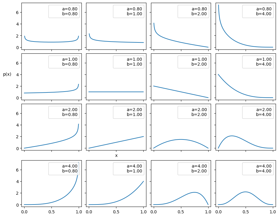
Part 2: Coin Example, Analytical Solution
Cell 2.1: Beta prior updated by streaming data
Goal:
- Watch a single Beta prior turn into a posterior as more coin-flip data arrives, one trial count at a time
prior=(1, 1)is uniform,(20, 20)looks Gaussian centered on 0.5,(1, 4)looks exponential centered near 0
Implementation: beta_prior_interactive()
- Generates binomial counts at each
n_trialsentry with_generate_data() - Plots the Beta(
a+y,b+N-y) posterior density for the trial count atIndex, steppable via the play button
hintros.print_obj_info(coin_ut.beta_prior_interactive)Usage
Inputs
seed: random seed for the generated datatheta (true): the true, otherwise-unknown success probabilityn_trials: comma-separated trial counts to step througha,b: the prior’s Beta shape parametersIndex/play button: whichn_trialsentry is shown
Panels
Posterior after N=... trials, y=... heads: the posterior density, withtheta (true)markedComments: current parameters and the resulting posterior distribution
coin_ut.beta_prior_interactive()Guided usage
- Set
a/bto1, 1(uniform prior), then stepIndexforward- Observe the posterior widen out then narrow around
theta (true)asNgrows
- Observe the posterior widen out then narrow around
- Compare
a/b=1, 1against20, 20at the sameIndex- Observe the strong
(20, 20)prior barely moves at lowN, while the uniform prior is dominated by the data almost immediately
- Observe the strong
Cell 2.2: Updating three priors at once
Goal:
- Compare three different Beta priors, uniform, Gaussian-like, and exponential-like, updated by the same growing dataset side by side
Implementation: update_prior()
- Fixes
theta_real = 0.35and a shared sequence ofn_trials/observed head counts - Plots all three priors’ posteriors at each trial count in one grid, so every prior can be compared at the same amount of data
coin_ut.update_prior()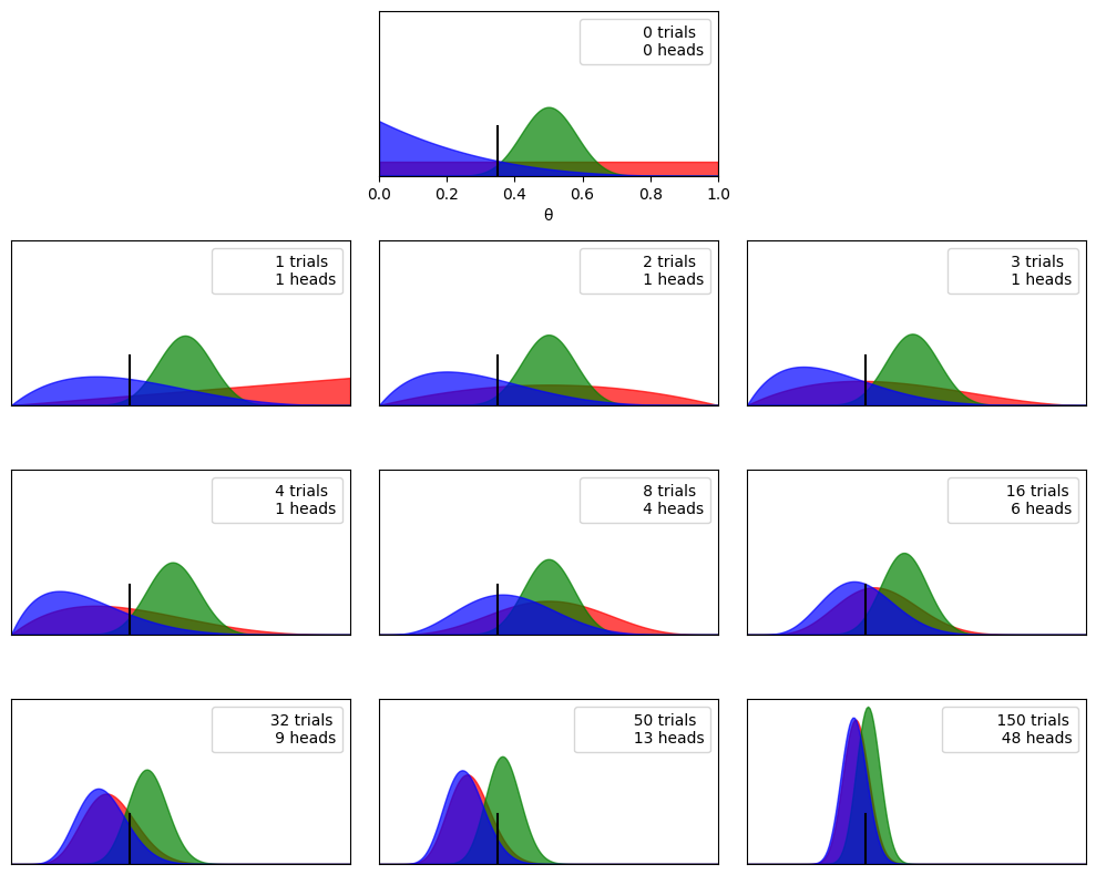
- All three posteriors converge toward the same spike at
theta_realasNgrows, regardless of how different the priors started - The Bayesian update replaces “guess and check” with an explicit rule for how a prior belief and new data combine into a posterior belief
Part 3: Coin Example, Numerical Solution
It’s a synthetic example!
- Assume you know the true value of (not true in general)
Workflow
- Model the prior and the likelihood
- Observe samples of the variable
- Run inference
- Generate samples of the posterior
- Summarize the posterior
- E.g., Highest-Posterior Density (HPD)
- Model the prior and the likelihood
Cell 3.1: Fitting the model with N=4
Goal:
- Fit the model above to
N=4synthetic observations, and read the fitted posterior witharviz’s trace, summary, rank-bar, and posterior plots
Implementation:
- Builds
model1with aBeta(1, 1)prior and aBernoullilikelihood observingdata1, then draws posterior samples withpm.sample()(PyMC’s NUTS sampler, 4 chains) az.plot_trace()/az.summary()/az.plot_posterior()summarize the resultingidata1
# Generate data from ground truth model.
np.random.seed(123)
n = 4
# Unknown value.
theta_real = 0.35
# Generate some observational data.
data1 = stats.bernoulli.rvs(p=theta_real, size=n)
print("data1=", data1)
array([1, 0, 0, 0])# Build PyMC model matching the mathematical model.
with pm.Model() as model1:
# Prior.
theta = pm.Beta("theta", alpha=1.0, beta=1.0)
# Likelihood.
y = pm.Bernoulli("y", p=theta, observed=data1)
# (Numerical) Inference to estimate the posterior distribution through samples.
idata1 = pm.sample(1000, random_seed=123)Auto-assigning NUTS sampler...
Initializing NUTS using jitter+adapt_diag...
Multiprocess sampling (4 chains in 4 jobs)
NUTS: [theta]
Sampling 4 chains for 1_000 tune and 1_000 draw iterations (4_000 + 4_000 draws total) took 1 seconds.
# Trace plot: one row per parameter, KDE (left) and chains (right).
az.plot_trace(idata1)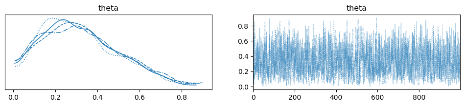
- No trace diverges, and the 4 chains mix well
- The KDE for
thetashould resemble a Beta density
# Numerical summary: mean, std dev, and HDI.
display(az.summary(idata1, kind="stats"))# Rank-bar diagnostic: flat bars indicate good mixing across chains.
az.plot_trace(idata1, kind="rank_bars", combined=True)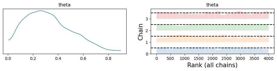
# Posterior density with the mean and HDI annotated.
az.plot_posterior(idata1)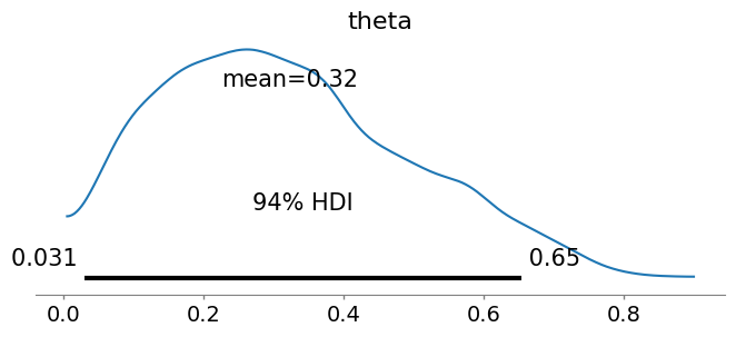
Cell 3.2: More data (N=20)
Goal:
- Repeat Cell 3.1 with
N=20observations, and see the posterior sharpen aroundtheta_realas more data arrives
Implementation:
- Same
Beta(1, 1)/Bernoullimodel asmodel1, refit on 20 observations asmodel2
np.random.seed(123)
n = 20
# Unknown value.
theta_real = 0.35
# Generate some observational data.
data2 = stats.bernoulli.rvs(p=theta_real, size=n)
print("data2=", data2)
array([1, 0, 0, 0, 1, 0, 1, 1, 0, 0, 0, 1, 0, 0, 0, 1, 0, 0, 0, 0])with pm.Model() as model2:
# Prior.
theta = pm.Beta("theta", alpha=1.0, beta=1.0)
# Likelihood.
y = pm.Bernoulli("y", p=theta, observed=data2)
# (Numerical) Inference to estimate the posterior distribution through samples.
idata2 = pm.sample(1000, random_seed=123)Auto-assigning NUTS sampler...
Initializing NUTS using jitter+adapt_diag...
Multiprocess sampling (4 chains in 4 jobs)
NUTS: [theta]
Sampling 4 chains for 1_000 tune and 1_000 draw iterations (4_000 + 4_000 draws total) took 1 seconds.
display(az.summary(idata2, kind="stats"))az.plot_posterior(idata2)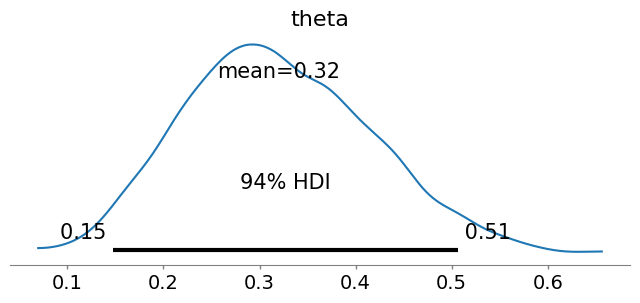
Cell 3.3: Even more data (N=100)
Goal:
- Repeat Cell 3.1 with
N=100observations, to see the posterior sharpen even further
Implementation:
- Same
Beta(1, 1)/Bernoullimodel asmodel1, refit on 100 observations asmodel3
np.random.seed(123)
n = 100
# Unknown value.
theta_real = 0.35
# Generate some observational data.
data3 = stats.bernoulli.rvs(p=theta_real, size=n)
print("data3=", data3)
array([1, 0, 0, 0, 1, 0, 1, 1, 0, 0, 0, 1, 0, 0, 0, 1, 0, 0, 0, 0, 0, 1,
1, 0, 1, 0, 0, 0, 0, 0, 0, 0, 0, 0, 0, 0, 0, 1, 1, 0, 0, 0, 0, 0,
1, 0, 0, 1, 0, 0, 0, 1, 0, 0, 0, 0, 0, 1, 1, 0, 1, 0, 0, 1, 1, 0,
1, 0, 0, 0, 0, 1, 0, 1, 0, 0, 0, 0, 0, 1, 0, 1, 0, 0, 1, 1, 0, 0,
0, 0, 1, 1, 0, 1, 0, 1, 0, 0, 0, 0])with pm.Model() as model3:
# Prior.
theta = pm.Beta("theta", alpha=1.0, beta=1.0)
# Likelihood.
y = pm.Bernoulli("y", p=theta, observed=data3)
# (Numerical) Inference to estimate the posterior distribution through samples.
idata3 = pm.sample(1000, random_seed=123)Auto-assigning NUTS sampler...
Initializing NUTS using jitter+adapt_diag...
Multiprocess sampling (4 chains in 4 jobs)
NUTS: [theta]
Sampling 4 chains for 1_000 tune and 1_000 draw iterations (4_000 + 4_000 draws total) took 1 seconds.
display(az.summary(idata3, kind="stats"))az.plot_posterior(idata3)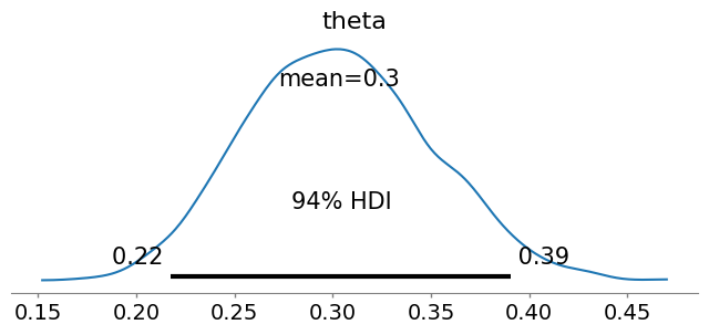
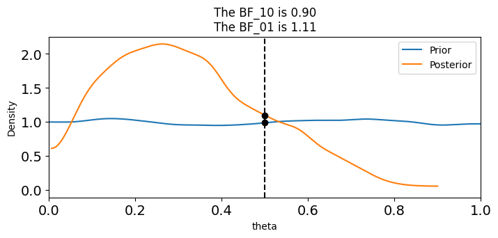
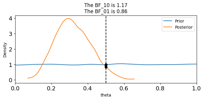
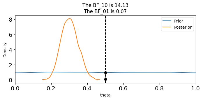
Cell 3.4: Savage-Dickey ratio
Goal:
- Test the point hypothesis against each of the three fitted posteriors via the Savage-Dickey density ratio
Implementation:
az.plot_bf()compares the posterior density atref_val=0.5against a uniform prior, foridata1,idata2, andidata3in turn
for idata in [idata1, idata2, idata3]:
    az.plot_bf(
        idata,
        var_name="theta",
        prior=np.random.uniform(0, 1, 10000),
        ref_val=0.5,
    )
    plt.xlim(0, 1)
arviz - WARNING - The reference value is outside of the posterior. This translate into infinite support for H1, which is most likely an overstatement.
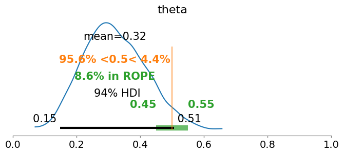
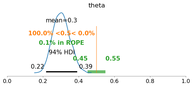
Cell 3.5: ROPE
Goal:
- Test whether plausibly equals 0.5 using a Region Of Practical Equivalence (ROPE) instead of a single point
Implementation:
az.plot_posterior()shades the[0.45, 0.55]ROPE and reports the fraction of the posterior it contains, for each fittedidata
for idata in [idata1, idata2, idata3]:
    az.plot_posterior(idata, rope=[0.45, 0.55], ref_val=0.5)
    plt.xlim(0, 1)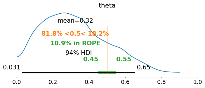
Part 4: Decision With a Loss Function
Cell 4.1: Minimizing a loss function
Goal:
- Turn a posterior into a point estimate by minimizing expected loss, instead of just reporting the posterior mean
Implementation: plot_loss(grid, loss_func)
- Plots the chosen
loss_func(squared, absolute, asymmetric, or sine) against a candidate-estimate grid
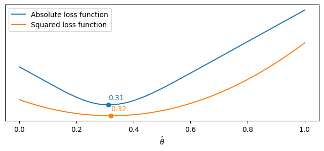
# loss_func = lambda x: coin_ut.squared_loss(x, theta_real)
# loss_func = lambda x: coin_ut.abs_loss(x, theta_real)
# loss_func = lambda x: coin_ut.asymmetric_loss(x, theta_real)
loss_func = lambda x: coin_ut.sin_loss(x, theta_real)

grid = np.linspace(-2.0, 2.0, 50)
coin_ut.plot_loss(grid, loss_func)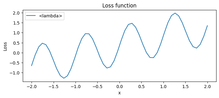
Cell 4.2: Posterior samples as a distribution
Goal:
- Look at the raw posterior draws for
thetadirectly: as a sequence, as a trace, and as a density
Implementation:
- Extracts the
thetacolumn fromidata1.to_dataframe()and plots it as a trace and a KDE
theta_draws = idata1.to_dataframe()[("posterior", "theta")]
display(theta_draws)
0 0.145339
1 0.146737
2 0.040329
3 0.109264
4 0.129498
...
3995 0.369080
3996 0.360284
3997 0.073147
3998 0.087704
3999 0.147956
Name: (posterior, theta), Length: 4000, dtype: float64plt.plot(theta_draws)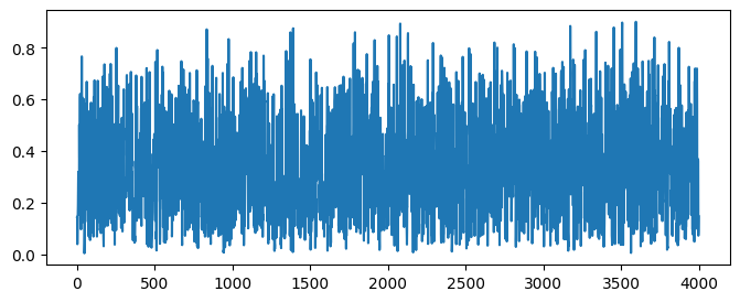
theta_draws.plot(kind="kde")<Axes: ylabel='Density'>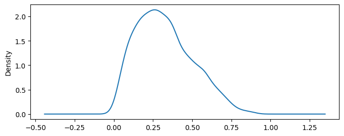
Cell 4.3: Picking the best theta
Goal:
- Combine the loss function from Cell 4.1 with the posterior samples to
pick the loss-minimizing point estimate, for both the
N=4andN=20posteriors
Implementation: pick_best_theta(idata)
- Searches over candidate
thetavalues and reports the one minimizing the expected loss under the posterior inidata
coin_ut.pick_best_theta(idata1)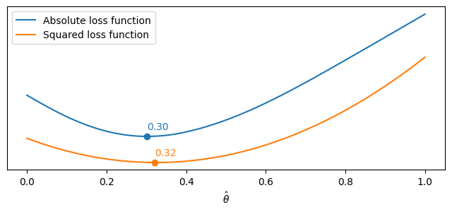
coin_ut.pick_best_theta(idata2)