Robust modeling - MSML610 -- Tutorials

Imports¶

%load_ext autoreload
%autoreload 2

!sudo /bin/bash -c "(source /venv/bin/activate; pip install --quiet graphviz)"

import arviz as az
import pymc as pm
import numpy as np
from IPython.display import display

import helpers.htutorial as ut
import L07_02_robust_modeling_utils as putils

ut.config_notebook()

dir_name = "./L07_data"
!ls $dir_name

Part 1: Chemical Shift¶

Cell 1.1: Loading the data¶

Goal:

Load the chemical-shift measurements used throughout this notebook

data = np.loadtxt(f"{dir_name}/chemical_shifts.csv")
print("len(data)=", len(data))
print("data=", data)

Cell 1.2: Visualizing the raw distribution¶

Goal:

Look at the data’s shape before fitting anything: it looks Gaussian, but with a couple of outliers

az.plot_kde(data, rug=True)
ut.process_figure("Chemical shift")

Cell 1.3: Fitting a Gaussian model¶

Goal:

Fit the data with the simplest reasonable model, a single Gaussian, as the baseline the Student-t model in Cell 1.7 will be compared against

Implementation:

mu ~ Uniform(40, 70) (wider than the data), sigma ~ HalfNormal(10), y ~ Normal(mu, sigma) observing data

with pm.Model() as model_g:
    # The mean is Uniform in [40, 70] (wider than the data).
    mu = pm.Uniform("mu", lower=40, upper=70)
    # The std dev is half normal with a wide scale relative to the data.
    sigma = pm.HalfNormal("sigma", sigma=10)
    # The model is N(mu, sigma).
    y = pm.Normal("y", mu=mu, sigma=sigma, observed=data)
    # Sample.
    idata_g = pm.sample(1000)

pm.model_to_graphviz(model_g)

Cell 1.4: Inspecting the Gaussian fit¶

Goal:

Check the sampling trace, the joint posterior of mu/sigma, and the numerical summary for the Gaussian fit

Implementation: az.plot_trace(), az.plot_pair(), az.summary()

# There are 4 traces for 2 variables.
az.plot_trace(idata_g)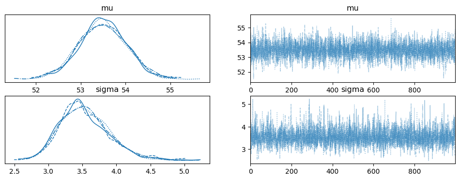

# The posterior distribution of the params is bi-dimensional: mu and sigma.
az.plot_pair(idata_g, kind="kde", marginals=True)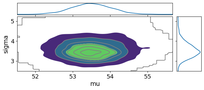

# Report a summary of the inference.
display(az.summary(idata_g, kind="stats").round(2))

Cell 1.5: Posterior predictive check for the Gaussian model¶

Goal:

Compare the observed data’s density against the Gaussian model’s posterior-predictive samples

Implementation: pm.sample_posterior_predictive(), az.plot_ppc()

Black: KDE of the observed data
Blue: KDEs of the posterior predictive samples
Orange: KDE of the posterior predictive mean

# Compute 100 posterior predictive samples.
y_pred_g = pm.sample_posterior_predictive(idata_g, model=model_g)

Sampling: [y]

az.plot_ppc(y_pred_g, mean=True, num_pp_samples=100)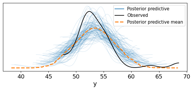

Cell 1.6: The Student-t distribution’s tails¶

Goal:

Show that the Student-t distribution approaches a Gaussian as its degrees of freedom nu grow, but keeps much heavier tails for small nu, which is what makes it robust to outliers

Implementation: plot_student_t_sweep(dfs, figsize=None)

Plots the Student-t PDF for nu in {0.1, 0.5, 1, 2, 5, 10, 30} next to the Gaussian (the nu -> infinity limit)

putils.plot_student_t_sweep()
ut.process_figure("Chap7: Student-t")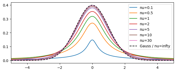

Cell 1.7: Fitting a Student-t model¶

Goal:

Refit the same data with a Student-t likelihood instead of a Gaussian, letting the model learn how heavy-tailed the noise should be

Implementation:

Same mu/sigma priors as model_g, plus nu ~ Exponential(1/30) (a nu around 30 is close to Gaussian); y ~ StudentT(mu, sigma, nu)

# Use a Student-t model.
with pm.Model() as model_t:
    mu = pm.Uniform("mu", 40, 75)
    sigma = pm.HalfNormal("sigma", sigma=10)
    # A Student-t with nu = 30 is close to a Gaussian.
    nu = pm.Exponential("nu", 1 / 30)
    #
    y = pm.StudentT("y", mu=mu, sigma=sigma, nu=nu, observed=data)
    idata_t = pm.sample(1_000)

Auto-assigning NUTS sampler...
Initializing NUTS using jitter+adapt_diag...
Multiprocess sampling (4 chains in 4 jobs)
NUTS: [mu, sigma, nu]

Sampling 4 chains for 1_000 tune and 1_000 draw iterations (4_000 + 4_000 draws total) took 2 seconds.

Cell 1.8: Inspecting the Student-t fit¶

Goal:

Check the sampling trace and numerical summary for the Student-t fit, the same diagnostics run on the Gaussian fit in Cell 1.4

az.plot_trace(idata_t)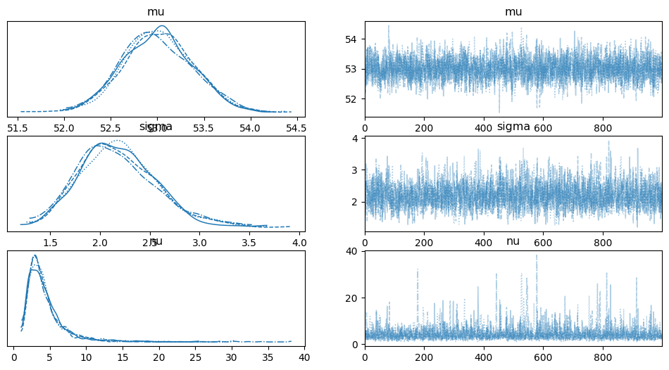

display(az.summary(idata_t, kind="stats").round(2))

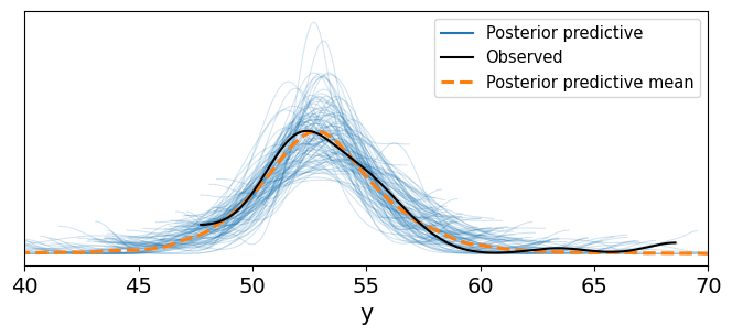
Cell 1.9: Posterior predictive check for the Student-t model¶

Goal:

Compare the Student-t model’s posterior-predictive fit against the data, and against the Gaussian model’s fit from Cell 1.5

Implementation: pm.sample_posterior_predictive(), az.plot_ppc()

# Compute 100 posterior predictive samples.
y_ppc_t = pm.sample_posterior_predictive(idata_t, model_t)

Sampling: [y]

ax = az.plot_ppc(y_ppc_t, num_pp_samples=100, mean=True)
ax.set_xlim(40, 70)