Probabilistic programming - MSML610 -- Tutorials

Imports¶

%load_ext autoreload
%autoreload 2

import arviz as az
import pandas as pd
import pymc as pm
import numpy as np
import scipy.stats as stats
import matplotlib.pyplot as plt
from IPython.display import display

import helpers.htutorial as ut
import L07_02_probabilistic_programming_utils as putils

ut.config_notebook()

Part 1: Posterior Predictive Checks¶

Cell 1.1: Loading and preparing the data¶

Goal:

Load a synthetic, mostly-linear dataset, and build the polynomial feature rows a linear and a quadratic model will each be fit on

Implementation:

Reads L07_data/dummy.csv, stacks x**i for i in 1..order, and standardizes both the features and the target to mean 0, std 1

dir_name = "./L07_data"
!ls $dir_name

# Load some data: it's mainly a linear relationship with some noise.
dummy_data = np.loadtxt(dir_name + "/dummy.csv")
x = dummy_data[:, 0]
y = dummy_data[:, 1]

# Transform the data applying various powers and stacking the data, so that
# we have different rows with different predicted variables.
order = 2
x_p = np.vstack([x**i for i in range(1, order + 1)])
display(pd.DataFrame(x_p))

# Normalize all the data.
x_c = (x_p - x_p.mean(axis=1, keepdims=True)) / x_p.std(axis=1, keepdims=True)
y_c = (y - y.mean()) / y.std()

Cell 1.2: Visualizing the raw relationship¶

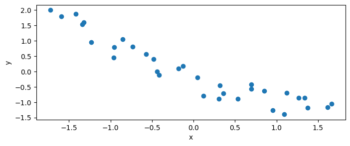
Goal:

Look at the order-0 feature (the raw, normalized x) against y before fitting anything

# Plot the 0-order data (i.e., the original one).
plt.scatter(x_c[0], y_c)
plt.xlabel("x")
plt.ylabel("y")
ut.save_plt("Lesson07.Comparing_models.data.png")

![](lectures_source/figures/Lesson07.Comparing_models.data.png)

Cell 1.3: Fitting linear and quadratic models¶

Goal:

Fit a linear and a quadratic Bayesian regression on the same data, so their posterior predictive fit can be compared

Implementation:

model_l: $\mu = \alpha + \beta x$ , model_p: $\mu = \alpha + \beta_1 x + \beta_2 x^2$ , both with a Normal likelihood and pm.sample()

# Linear model.
with pm.Model() as model_l:
    # mu = alpha + beta * x
    alpha = pm.Normal("alpha", mu=0, sigma=1)
    beta = pm.Normal("beta", mu=0, sigma=10)
    mu = alpha + beta * x_c[0]
    #
    sigma = pm.HalfNormal("sigma", 5)
    #
    y_pred = pm.Normal("y_pred", mu=mu, sigma=sigma, observed=y_c)
    #
    idata_l = pm.sample(2000, idata_kwargs={"log_likelihood": True})
    idata_l = pm.sample_posterior_predictive(idata_l, extend_inferencedata=True)

# Quadratic model.
with pm.Model() as model_p:
    # mu = alpha + beta_1 * x + beta_2 * x^2
    alpha = pm.Normal("alpha", mu=0, sigma=1)
    # Beta is a 2-dim vector.
    beta = pm.Normal("beta", mu=0, sigma=10, shape=order)
    mu = alpha + pm.math.dot(beta, x_c)
    #
    sigma = pm.HalfNormal("sigma", 5)
    #
    y_pred = pm.Normal("y_pred", mu=mu, sigma=sigma, observed=y_c)
    #
    idata_q = pm.sample(2000, idata_kwargs={"log_likelihood": True})
    idata_q = pm.sample_posterior_predictive(idata_q, extend_inferencedata=True)

Auto-assigning NUTS sampler...
Initializing NUTS using jitter+adapt_diag...
Multiprocess sampling (4 chains in 4 jobs)
NUTS: [alpha, beta, sigma]

Sampling 4 chains for 1_000 tune and 2_000 draw iterations (4_000 + 8_000 draws total) took 1 seconds.
Sampling: [y_pred]

Auto-assigning NUTS sampler...
Initializing NUTS using jitter+adapt_diag...
Multiprocess sampling (4 chains in 4 jobs)
NUTS: [alpha, beta, sigma]

Sampling 4 chains for 1_000 tune and 2_000 draw iterations (4_000 + 8_000 draws total) took 2 seconds.
Sampling: [y_pred]

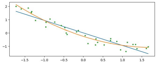
Cell 1.4: Comparing the fitted models against the data¶

Goal:

Plot both models’ mean-posterior curve against the data, to see the difference a quadratic term makes

Implementation:

Extracts posterior means for alpha/beta from each idata via az.extract(), then evaluates each curve over a dense x grid

# Sample the x space uniformly with 100 samples.
x_new = np.linspace(x_c[0].min(), x_c[0].max(), 100)

# Posterior.
posterior_l = az.extract(idata_l)
posterior_p = az.extract(idata_q)

# Compute the mean posterior of the linear model.
alpha_l_post = posterior_l["alpha"].mean().item()
beta_l_post = posterior_l["beta"].mean().item()
print(
    f"linear model: alpha_l_post={alpha_l_post:.2g}, beta_l_post={beta_l_post:.2g}"
)
y_l_post = alpha_l_post + beta_l_post * x_new

# Plot the mean posterior of the linear model.
plt.plot(x_new, y_l_post, "C0", label="linear model")

# Quadratic model.
alpha_p_post = posterior_p["alpha"].mean().item()
beta_p_post = posterior_p["beta"].mean("sample")
print(
    f"quadratic model: alpha_p_post={alpha_p_post:.2g}, "
    f"beta_post[0]={beta_p_post[0]:.2g}, beta_post[1]={beta_p_post[1]:.2g}"
)
y_p_post = alpha_p_post + np.dot(beta_p_post, x_c)
plt.plot(x_c[0], y_p_post, "C1", label="quadratic model")

# Plot data.
plt.plot(x_c[0], y_c, "C2.")
ut.save_plt("Lesson07.Comparing_models.model_fit.png")

linear model: alpha_l_post=-0.00096, beta_l_post=-0.94
quadratic model: alpha_p_post=-0.00017, beta_post[0]=-1.5, beta_post[1]=0.56
![](lectures_source/figures/Lesson07.Comparing_models.model_fit.png)

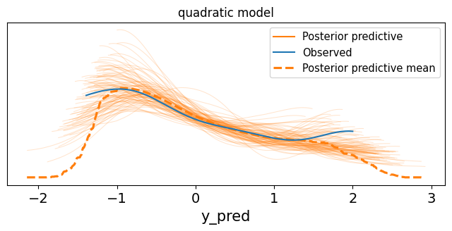
Cell 1.5: Posterior predictive check plots¶

Goal:

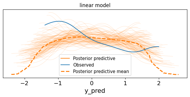
Check each model’s fit by comparing its posterior-predictive samples against the observed data

Implementation: az.plot_ppc(idata, num_pp_samples=100, ...)

Overlays 100 posterior-predictive draws on the observed data’s density, for the linear and the quadratic model in turn

az.plot_ppc(idata_l, num_pp_samples=100, colors=["C1", "C0", "C1"])
plt.title("linear model")
ut.save_plt("Lesson07.Comparing_models.lin_model_PPC.png")

az.plot_ppc(idata_q, num_pp_samples=100, colors=["C1", "C0", "C1"])
plt.title("quadratic model")
ut.save_plt("Lesson07.Comparing_models.quadr_model_PPC.png")

![](lectures_source/figures/Lesson07.Comparing_models.lin_model_PPC.png)
![](lectures_source/figures/Lesson07.Comparing_models.quadr_model_PPC.png)

Cell 1.6: Bayesian p-value for a statistic¶

Goal:

Compare the Bayesian p-value of the mean and of the interquartile range (IQR), for both models, as two different test statistics

Implementation: az.plot_bpv(idata, kind="t_stat", t_stat=...)

t_stat="mean" uses the built-in mean statistic; t_stat=putils.iqr plugs in the custom IQR statistic from the utils file

colors = ["C0", "C1"]
idatas = [idata_l, idata_q]
fig, axes = plt.subplots(2, 1)

# Plot the Bayesian p-value for the mean, for both models.
for idata, c in zip(idatas, colors):
    az.plot_bpv(idata, kind="t_stat", t_stat="mean", ax=axes[0], color=c)
    axes[0].set_title("linear")

# Plot the Bayesian p-value for the interquartile range, for both models.
for idata, c in zip(idatas, colors):
    az.plot_bpv(idata, kind="t_stat", t_stat=putils.iqr, ax=axes[1], color=c)

Cell 1.7: Bayesian p-value for the entire distribution¶

Goal:

Compare the Bayesian p-value across the entire predictive distribution, not just one summary statistic

fig, ax = plt.subplots()
for idata, c in zip(idatas, colors):
    az.plot_bpv(idata, color=c, ax=ax)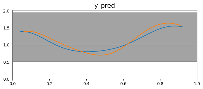

Part 2: Overfitting¶

Cell 2.1: In-sample vs out-of-sample data¶

Goal:

Set up a small in-sample dataset and a separate out-of-sample dataset, used next to show how model complexity trades off against overfitting

x0 = np.array([4.0, 5.0, 6.0, 9.0, 12, 14.0])
y0 = np.array([4.2, 6.1, 5.0, 10.0, 10, 14.0])
x1 = np.array([6.5, 10])
y1 = np.array([7, 10])

_, ax = plt.subplots(1, 1)
ax.plot(x0, y0, "ko")
_ = ax.plot(x1, y1, "rs")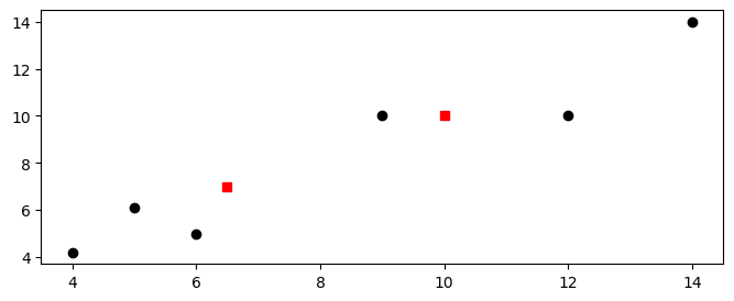

Cell 2.2: Fitting polynomial models of increasing order¶

Goal:

Fit polynomials of order 0, 1, and 5 on the in-sample data, and read off each one’s $R^2$

Implementation: putils.plot_models(ax, x_n, x0, y0, order, ps)

Fits each order with np.polynomial.Polynomial.fit(), then plots the fitted curve and its $R^2$ against (x0, y0)

_, ax = plt.subplots(1, 1)
ax.plot(x0, y0, "ko", zorder=3)

# Learn 3 models.
order_list = [0, 1, 5]
x_n = np.linspace(x0.min(), x0.max(), 100)
ps = [np.polynomial.Polynomial.fit(x0, y0, deg=i) for i in order_list]
putils.plot_models(ax, x_n, x0, y0, order_list, ps)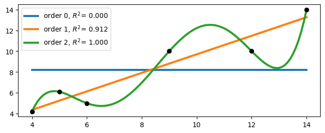

Cell 2.3: Evaluating the fit on out-of-sample data¶

Goal:

Score the same 3 fitted models against the combined in-sample plus out-of-sample data, to see which order actually generalizes

Implementation: putils.plot_models(...), now scored against the combined dataset instead of only the in-sample one

_, ax = plt.subplots(figsize=(12, 4))
ax.plot(x0, y0, "ko", zorder=3)
ax.plot(x1, y1, "rs", zorder=3)

x_all = np.concatenate((x0, x1))
y_all = np.concatenate((y0, y1))
putils.plot_models(ax, x_n, x_all, y_all, order_list, ps)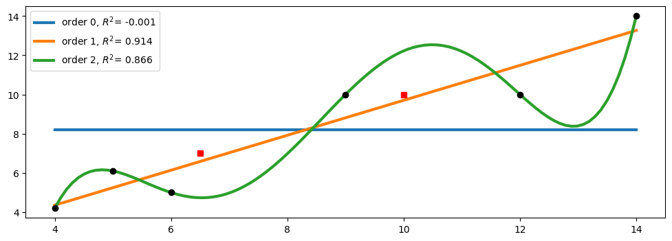

Cell 2.4: Calculating predictive accuracy¶

Goal:

Compute two out-of-sample predictive-accuracy estimates, WAIC and PSIS- LOO, for the linear and quadratic Bayesian models from Part 1

Implementation: az.waic(idata) and az.loo(idata)

waic_l = az.waic(idata_l)
display(waic_l)

Computed from 8000 posterior samples and 33 observations log-likelihood matrix.

          Estimate       SE
elpd_waic   -14.38     2.67
p_waic        2.45        -

waic_q = az.waic(idata_q)
display(waic_q)

Computed from 8000 posterior samples and 33 observations log-likelihood matrix.

          Estimate       SE
elpd_waic    -4.53     2.33
p_waic        2.61        -

loo_l = az.loo(idata_l)
display(loo_l)

Computed from 8000 posterior samples and 33 observations log-likelihood matrix.

         Estimate       SE
elpd_loo   -14.41     2.67
p_loo        2.48        -
------

Pareto k diagnostic values:
                         Count   Pct.
(-Inf, 0.70]   (good)       33  100.0%
   (0.70, 1]   (bad)         0    0.0%
   (1, Inf)   (very bad)    0    0.0%

loo_q = az.loo(idata_q)
display(loo_q)

Computed from 8000 posterior samples and 33 observations log-likelihood matrix.

         Estimate       SE
elpd_loo    -4.56     2.33
p_loo        2.64        -
------

Pareto k diagnostic values:
                         Count   Pct.
(-Inf, 0.70]   (good)       33  100.0%
   (0.70, 1]   (bad)         0    0.0%
   (1, Inf)   (very bad)    0    0.0%

Part 3: Comparing and Averaging Models¶

Cell 3.1: Comparing models¶

Goal:

Rank the linear and quadratic model by predictive accuracy, with az.compare()'s standard-error-aware comparison

Implementation: az.compare({...}), then az.plot_compare()

cmp_df = az.compare({"model_l": idata_l, "model_q": idata_q})
display(cmp_df)

_ = az.plot_compare(cmp_df)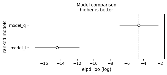

Cell 3.2: Model averaging¶

Goal:

Combine both models’ posterior predictive distributions into one weighted mixture, instead of picking a single “best” model

Implementation: az.weight_predictions(idatas, weights)

Weights the linear and quadratic posterior predictive by 0.35/0.65, then compares all three predictive densities via az.plot_kde()

idatas = [idata_l, idata_q]
weights = [0.35, 0.65]
idata_w = az.weight_predictions(idatas, weights)

# Plot the KDE of the posterior predictive for each model, and the mixture.
_, ax = plt.subplots(figsize=(10, 6))

az.plot_kde(
    idata_l.posterior_predictive["y_pred"].values,
    plot_kwargs={"color": "C0", "lw": 3},
    label="linear",
    ax=ax,
)
az.plot_kde(
    idata_q.posterior_predictive["y_pred"].values,
    plot_kwargs={"color": "C1", "lw": 3},
    label="quadratic",
    ax=ax,
)
az.plot_kde(
    idata_w.posterior_predictive["y_pred"].values,
    plot_kwargs={"color": "C2", "lw": 3, "ls": "--"},
    label="weighted",
    ax=ax,
)
_ = plt.legend()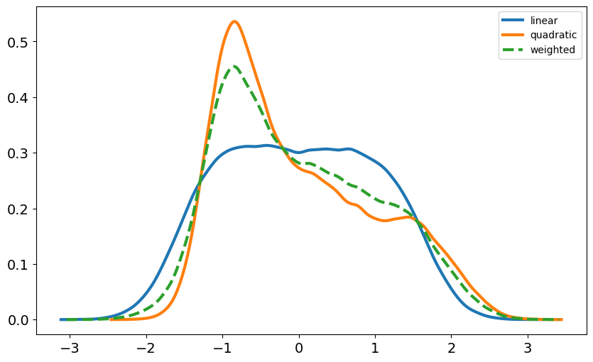

Part 4: Mixture Models¶

Cell 4.1: Marginalization over a Gaussian mixture¶

Goal:

Fit a 2-component Gaussian mixture to chemical-shift data, marginalizing over a discrete latent component label for every point

Implementation:

p ~ Dirichlet([1, 1]) picks the mixture weights, z ~ Categorical(p) assigns each point a component, and y | z ~ Normal(means[z], sd) is the observed likelihood; all three are estimated jointly

!ls $dir_name

anscombe.csv	     chemical_shifts_theo_exp.csv  islands.csv
anscombe_3.csv	     coal.csv			   penguins.csv
babies.csv	     dummy.csv			   pigs.csv
bikes.csv	     fish.csv			   redwood.csv
bikes_full.csv	     football_players.csv	   space_flu.csv
body_fat.csv	     horseshoe_crab.csv		   tips.csv
body_fat_full.csv    howell.csv
chemical_shifts.csv  iris.csv

cs = pd.read_csv(dir_name + "/chemical_shifts_theo_exp.csv")
cs_exp = pd.DataFrame(cs["exp"])
display(cs_exp.head())
print("shape=", len(cs_exp))

shape= 1776

_, ax = plt.subplots()
_ = plt.hist(cs_exp, density=True, bins=30, alpha=0.3)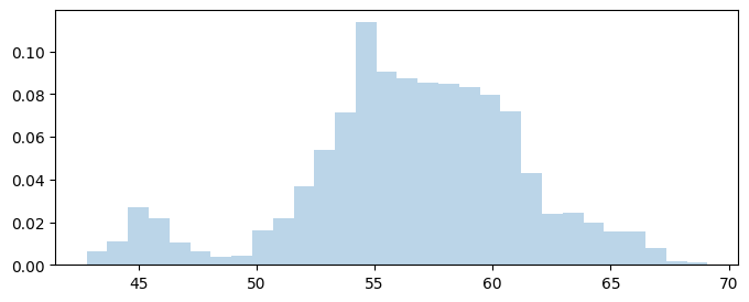

# The parameters to estimate are:
# - a latent variable (one component per data point) drawn from a Dirichlet
#   - All vars are estimated together as one hierarchical model.
# - the means and shared std dev of the 2 Gaussian components
K = 2
with pm.Model() as model_kg:
    # Prior p ~ Dirichlet([1, 1]), which is a Beta.
    p = pm.Dirichlet("p", a=np.ones(K))
    # Assign each data point a component via the latent variable "z".
    z = pm.Categorical("z", p=p, shape=len(cs_exp))
    # 2 Gaussians with different mean and same std.
    means = pm.Normal("means", mu=cs_exp.mean(), sigma=10, shape=K)
    sd = pm.HalfNormal("sd", sigma=10)
    # The distribution is a Gaussian whose mean is a function of z.
    y = pm.Normal("y", mu=means[z], sigma=sd, observed=cs_exp)
    trace_kg = pm.sample()

Multiprocess sampling (4 chains in 4 jobs)
CompoundStep
>NUTS: [p, means, sd]
>BinaryGibbsMetropolis: [z]

---------------------------------------------------------------------------
ValueError                                Traceback (most recent call last)
Cell In[73], line 16
     14 # The distribution is a Gaussian whose means are function of the latent variable.
     15 y = pm.Normal("y", mu=means[z], sigma=sd, observed=cs_exp)
---> 16 trace_kg = pm.sample()

File /venv/lib/python3.12/site-packages/pymc/sampling/mcmc.py:891, in sample(draws, tune, chains, cores, random_seed, progressbar, progressbar_theme, step, var_names, nuts_sampler, initvals, init, jitter_max_retries, n_init, trace, discard_tuned_samples, compute_convergence_checks, keep_warning_stat, return_inferencedata, idata_kwargs, nuts_sampler_kwargs, callback, mp_ctx, blas_cores, model, **kwargs)
    887 t_sampling = time.time() - t_start
    889 # Packaging, validating and returning the result was extracted
    890 # into a function to make it easier to test and refactor.
--> 891 return _sample_return(
    892     run=run,
    893     traces=traces,
    894     tune=tune,
    895     t_sampling=t_sampling,
    896     discard_tuned_samples=discard_tuned_samples,
    897     compute_convergence_checks=compute_convergence_checks,
    898     return_inferencedata=return_inferencedata,
    899     keep_warning_stat=keep_warning_stat,
    900     idata_kwargs=idata_kwargs or {},
    901     model=model,
    902 )

File /venv/lib/python3.12/site-packages/pymc/sampling/mcmc.py:924, in _sample_return(run, traces, tune, t_sampling, discard_tuned_samples, compute_convergence_checks, return_inferencedata, keep_warning_stat, idata_kwargs, model)
    922 # Pick and slice chains to keep the maximum number of samples
    923 if discard_tuned_samples:
--> 924     traces, length = _choose_chains(traces, tune)
    925 else:
    926     traces, length = _choose_chains(traces, 0)

File /venv/lib/python3.12/site-packages/pymc/backends/base.py:603, in _choose_chains(traces, tune)
    601 lengths = [max(0, len(trace) - tune) for trace in traces]
    602 if not sum(lengths):
--> 603     raise ValueError("Not enough samples to build a trace.")
    605 idxs = np.argsort(lengths)
    606 l_sort = np.array(lengths)[idxs]

ValueError: Not enough samples to build a trace.

varnames = ["means", "p"]
_ = az.plot_trace(trace_kg, varnames)

Part 5: Inference Engines¶

Cell 5.1: Grid approximation¶

Goal:

Estimate a coin-flip posterior by brute-force grid approximation: a uniform prior times a Binomial likelihood, normalized over a grid

Implementation: putils.posterior_grid(grid_points, heads, tails)

heads = 3
tails = 10
grid_points = 20

print("heads=", heads)
print("tails=", tails)
grid, prior, likelihood, posterior = putils.posterior_grid(
    grid_points, heads, tails
)

# Plot posterior.
plt.plot(grid, prior, label="prior")
plt.plot(grid, likelihood, label="likelihood")
plt.plot(grid, posterior, label="posterior")
_ = plt.legend()

Cell 5.2: Monte Carlo estimate of pi¶

Goal:

Estimate pi by the classic dartboard Monte Carlo method: the fraction of random points inside the unit circle approximates pi/4

Implementation:

Draws N uniform 2D points in $[-1, 1]^2$ and checks which fall inside the unit circle

N = 10000
x_mc, y_mc = np.random.uniform(-1, 1, size=(2, N))
inside = (x_mc**2 + y_mc**2) <= 1
pi_estimate = inside.sum() * 4 / N
error = abs((pi_estimate - np.pi) / pi_estimate) * 100
outside = np.invert(inside)

plt.figure(figsize=(8, 8))
plt.plot(x_mc[inside], y_mc[inside], "b.")
plt.plot(x_mc[outside], y_mc[outside], "r.")
plt.plot(0, 0, label=f"pi*= {pi_estimate:4.3f}\nerror = {error:4.3f}", alpha=0)
plt.axis("square")
plt.xticks([])
plt.yticks([])
_ = plt.legend(loc=1, frameon=True, framealpha=0.9)

Cell 5.3: Metropolis sampler¶

Goal:

Implement the Metropolis algorithm from scratch, and check that it recovers a known Beta(2, 5) target density

Implementation: putils.metropolis(func, draws)

Proposes a Gaussian random-walk step, accepts it with probability min(1, new_prob / old_prob), and repeats it otherwise

np.random.seed(3)
func = stats.beta(2, 5)
trace = putils.metropolis(func=func)
x_grid = np.linspace(0.01, 0.99, 100)
y_grid = func.pdf(x_grid)
plt.xlim(0, 1)
plt.plot(x_grid, y_grid, "C1-", lw=3, label="True distribution")
plt.hist(trace[trace > 0], bins=25, density=True, label="Estimated distribution")
plt.xlabel("x")
plt.ylabel("pdf(x)")
plt.yticks([])
plt.legend()
plt.savefig("B11197_08_05.png")

Part 6: Diagnosing Convergence¶

Cell 6.1: Centered vs non-centered parametrization¶

Goal:

Fit the same hierarchical model in two equivalent parametrizations, centered and non-centered, and compare their sampling traces

Implementation:

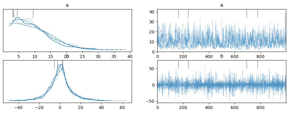
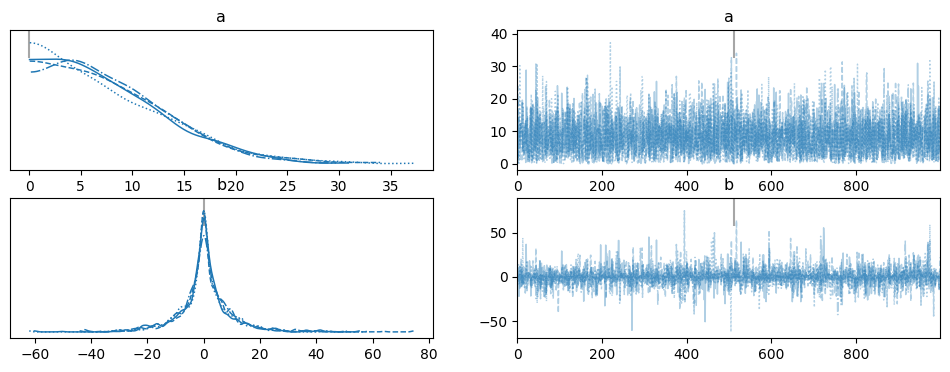
model_c: b ~ Normal(0, a) directly (centered)
model_nc: b = b_offset * a with b_offset ~ Normal(0, 1) (non-centered, easier for NUTS to sample when a is small)

# Centered model.
with pm.Model() as model_c:
    # Param for the std dev of all Gaussians.
    a = pm.HalfNormal("a", 10)
    # 10 normals with mean=0 and std dev=a.
    b = pm.Normal("b", 0, a, shape=10)
    idata_c = pm.sample(random_seed=73)

Auto-assigning NUTS sampler...
Initializing NUTS using jitter+adapt_diag...
Multiprocess sampling (4 chains in 4 jobs)
NUTS: [a, b]

Sampling 4 chains for 1_000 tune and 1_000 draw iterations (4_000 + 4_000 draws total) took 2 seconds.
There were 4 divergences after tuning. Increase `target_accept` or reparameterize.
The rhat statistic is larger than 1.01 for some parameters. This indicates problems during sampling. See https://arxiv.org/abs/1903.08008 for details
The effective sample size per chain is smaller than 100 for some parameters.  A higher number is needed for reliable rhat and ess computation. See https://arxiv.org/abs/1903.08008 for details

coords = {"b_dim_0": [0]}
_ = az.plot_trace(
    idata_c, var_names=["a", "b"], coords=coords, divergences="top"
)

# Non-centered (re-parametrized) model.
with pm.Model() as model_nc:
    a = pm.HalfNormal("a", 10)
    b_offset = pm.Normal("b_offset", mu=0, sigma=1, shape=10)
    # Gaussians are rescaled.
    b = pm.Deterministic("b", 0 + b_offset * a)
    idata_nc = pm.sample(random_seed=73)

Auto-assigning NUTS sampler...
Initializing NUTS using jitter+adapt_diag...
Multiprocess sampling (4 chains in 4 jobs)
NUTS: [a, b_offset]

Sampling 4 chains for 1_000 tune and 1_000 draw iterations (4_000 + 4_000 draws total) took 1 seconds.
There were 1 divergences after tuning. Increase `target_accept` or reparameterize.

ax = az.plot_trace(
    idata_nc, var_names=["a", "b"], coords=coords, divergences="top"
)

Cell 6.2: Rank plots¶

Goal:

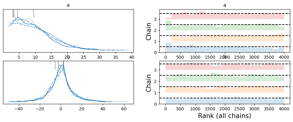
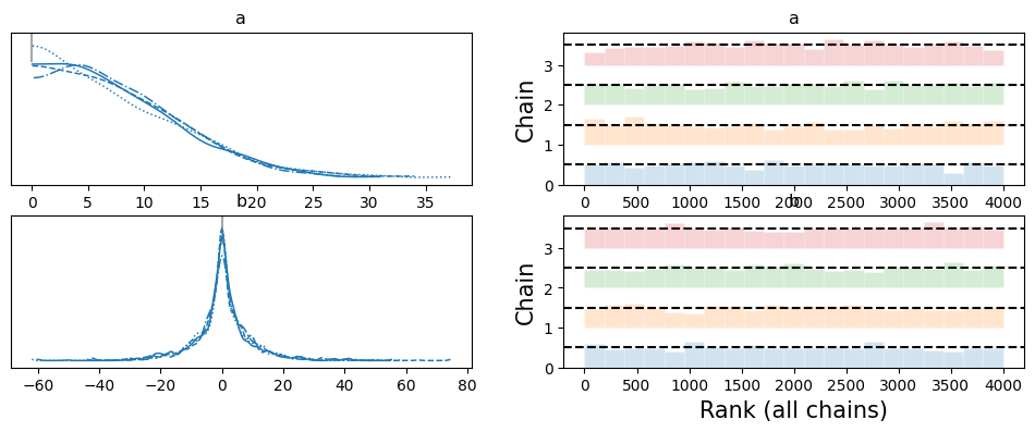
Read the same centered-vs-non-centered comparison off rank plots, a diagnostic that is easier to read than overlaid trace lines for many chains

Implementation: az.plot_trace(idata, kind="rank_bars", ...)

_ = az.plot_trace(
    idata_c,
    var_names=["a", "b"],
    divergences="top",
    kind="rank_bars",
    coords=coords,
)

_ = az.plot_trace(
    idata_nc,
    var_names=["a", "b"],
    divergences="top",
    kind="rank_bars",
    coords=coords,
)

Cell 6.3: R-hat¶

Goal:

Compare the centered and non-centered fits’ summary statistics and R-hat convergence diagnostic side by side

summaries = pd.concat(
    [az.summary(idata_c, var_names=["a"]), az.summary(idata_nc, var_names=["a"])]
)
summaries.index = ["centered", "non_centered"]
display(summaries)

display(az.rhat(idata_c, var_names="a b".split()).to_dataframe().T)

display(az.rhat(idata_nc, var_names="a b".split()).to_dataframe().T)

Cell 6.4: Effective sample size (ESS)¶

Goal:

Compare autocorrelation and effective sample size between the two parametrizations: the non-centered one should mix better

_ = az.plot_autocorr(idata_c, var_names=["a"])

display(az.ess(idata_c, var_names="a b".split()).to_dataframe().T)

_ = az.plot_autocorr(idata_nc, var_names=["a"])

display(az.ess(idata_nc, var_names="a b".split()).to_dataframe().T)

# Plot the ESS by quantile.
az.plot_ess(idata_c, var_names="a", kind="quantile")
_ = az.plot_ess(idata_nc, var_names="a", kind="quantile")

az.plot_ess(idata_c, var_names="a", kind="evolution")
_ = az.plot_ess(idata_nc, var_names="a", kind="evolution")

Cell 6.5: Divergences¶

Goal:

Visualize where divergent transitions land in parameter space, for both parametrizations, and check a’s marginal for both at once

Implementation: az.plot_pair(..., divergences=True) and az.plot_parallel()

_, ax = plt.subplots(
    1, 2, sharey=True, sharex=True, figsize=(10, 5), constrained_layout=True
)
for idx, tr in enumerate([idata_c, idata_nc]):
    az.plot_pair(
        tr,
        var_names=["b", "a"],
        coords={"b_dim_0": [0]},
        kind="scatter",
        divergences=True,
        divergences_kwargs={"color": "C1"},
        ax=ax[idx],
    )
    ax[idx].set_title(["centered", "non-centered"][idx])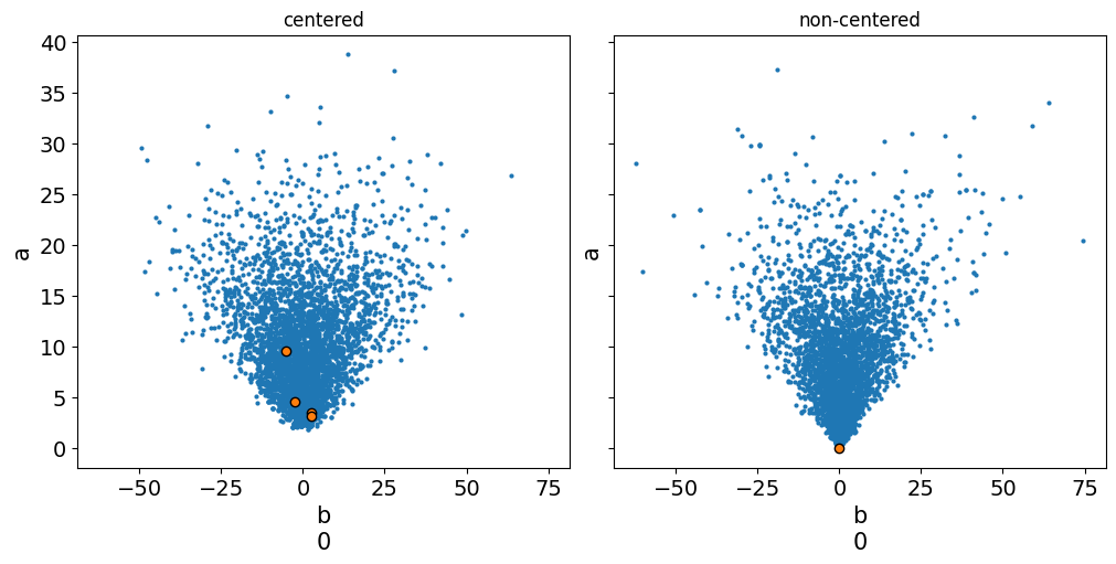

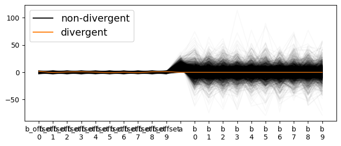
_ = az.plot_parallel(idata_c)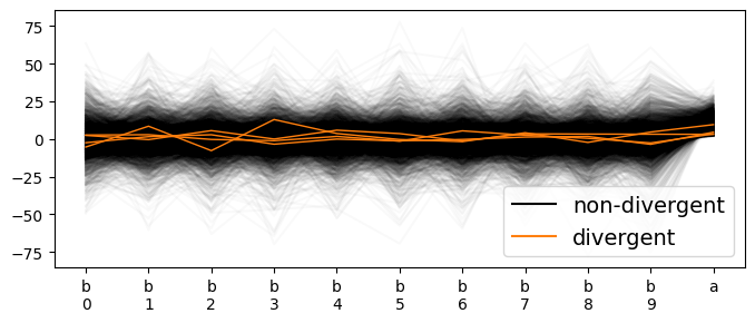

_ = az.plot_parallel(idata_nc)

<Axes: >