Imports
%load_ext autoreload
%autoreload 2

import arviz as az
import pandas as pd
import pymc as pm
import numpy as np
import matplotlib.pyplot as plt
from IPython.display import display
import helpers.htutorial as ut
import L07_05_evaluating_models_utils as putils
ut.config_notebook()
dir_name = "./L07_data"
!ls $dir_namePart 1: Posterior Predictive Check Examples
Cell 1.1: Loading and transforming the data
Goal:
- Load a near-linear synthetic dataset, and expand it into powers of
xso a linear and a quadratic model can be fit on the same feature matrix
Implementation:
x_pstacksx**1,x**2; bothx_pandyare then standardized to zero mean, unit variance
dummy_data = np.loadtxt(dir_name + "/dummy.csv")
x = dummy_data[:, 0]
y = dummy_data[:, 1]

# Transform the data applying various powers and stacking the data, so that
# we have different rows with different predicted variables.
order = 2
x_p = np.vstack([x**i for i in range(1, order + 1)])
display(pd.DataFrame(x_p))

# Normalize all the data.
x_c = (x_p - x_p.mean(axis=1, keepdims=True)) / x_p.std(axis=1, keepdims=True)
y_c = (y - y.mean()) / y.std()
Cell 1.2: Visualizing the raw data
Goal:
- Plot the (0th-order, i.e., original) standardized data before fitting
plt.scatter(x_c[0], y_c)
plt.xlabel("x")
plt.ylabel("y")
ut.save_plt("Lesson07.Comparing_models.data.png")
Loading...
---------------------------------------------------------------------------
FileNotFoundError                         Traceback (most recent call last)
Cell In[5], line 21
     18 plt.xlabel('x')
     19 plt.ylabel('y');
---> 21 ut.save_plt("Lesson07.Comparing_models.data.png")

File /app/msml610/tutorials/msml610_utils.py:757, in save_plt(file_name)
    755 def save_plt(file_name):
    756     file_name = os.path.join(fig_dir, file_name)
--> 757     plt.savefig(file_name, dpi=300, bbox_inches="tight")
    758     #
    759     file_name = file_name.replace("/app/", "")

File /venv/lib/python3.12/site-packages/matplotlib/pyplot.py:1251, in savefig(*args, **kwargs)
   1248 fig = gcf()
   1249 # savefig default implementation has no return, so mypy is unhappy
   1250 # presumably this is here because subclasses can return?
-> 1251 res = fig.savefig(*args, **kwargs)  # type: ignore[func-returns-value]
   1252 fig.canvas.draw_idle()  # Need this if 'transparent=True', to reset colors.
   1253 return res

File /venv/lib/python3.12/site-packages/matplotlib/figure.py:3490, in Figure.savefig(self, fname, transparent, **kwargs)
   3488     for ax in self.axes:
   3489         _recursively_make_axes_transparent(stack, ax)
-> 3490 self.canvas.print_figure(fname, **kwargs)

File /venv/lib/python3.12/site-packages/matplotlib/backend_bases.py:2184, in FigureCanvasBase.print_figure(self, filename, dpi, facecolor, edgecolor, orientation, format, bbox_inches, pad_inches, bbox_extra_artists, backend, **kwargs)
   2180 try:
   2181     # _get_renderer may change the figure dpi (as vector formats
   2182     # force the figure dpi to 72), so we need to set it again here.
   2183     with cbook._setattr_cm(self.figure, dpi=dpi):
-> 2184         result = print_method(
   2185             filename,
   2186             facecolor=facecolor,
   2187             edgecolor=edgecolor,
   2188             orientation=orientation,
   2189             bbox_inches_restore=_bbox_inches_restore,
   2190             **kwargs)
   2191 finally:
   2192     if bbox_inches and restore_bbox:

File /venv/lib/python3.12/site-packages/matplotlib/backend_bases.py:2040, in FigureCanvasBase._switch_canvas_and_return_print_method.<locals>.<lambda>(*args, **kwargs)
   2036     optional_kws = {  # Passed by print_figure for other renderers.
   2037         "dpi", "facecolor", "edgecolor", "orientation",
   2038         "bbox_inches_restore"}
   2039     skip = optional_kws - {*inspect.signature(meth).parameters}
-> 2040     print_method = functools.wraps(meth)(lambda *args, **kwargs: meth(
   2041         *args, **{k: v for k, v in kwargs.items() if k not in skip}))
   2042 else:  # Let third-parties do as they see fit.
   2043     print_method = meth

File /venv/lib/python3.12/site-packages/matplotlib/backends/backend_agg.py:481, in FigureCanvasAgg.print_png(self, filename_or_obj, metadata, pil_kwargs)
    434 def print_png(self, filename_or_obj, *, metadata=None, pil_kwargs=None):
    435     """
    436     Write the figure to a PNG file.
    437
   (...)
    479         *metadata*, including the default 'Software' key.
    480     """
--> 481     self._print_pil(filename_or_obj, "png", pil_kwargs, metadata)

File /venv/lib/python3.12/site-packages/matplotlib/backends/backend_agg.py:430, in FigureCanvasAgg._print_pil(self, filename_or_obj, fmt, pil_kwargs, metadata)
    425 """
    426 Draw the canvas, then save it using `.image.imsave` (to which
    427 *pil_kwargs* and *metadata* are forwarded).
    428 """
    429 FigureCanvasAgg.draw(self)
--> 430 mpl.image.imsave(
    431     filename_or_obj, self.buffer_rgba(), format=fmt, origin="upper",
    432     dpi=self.figure.dpi, metadata=metadata, pil_kwargs=pil_kwargs)

File /venv/lib/python3.12/site-packages/matplotlib/image.py:1657, in imsave(fname, arr, vmin, vmax, cmap, format, origin, dpi, metadata, pil_kwargs)
   1655 pil_kwargs.setdefault("format", format)
   1656 pil_kwargs.setdefault("dpi", (dpi, dpi))
-> 1657 image.save(fname, **pil_kwargs)

File /venv/lib/python3.12/site-packages/PIL/Image.py:2576, in Image.save(self, fp, format, **params)
   2574         fp = builtins.open(filename, "r+b")
   2575     else:
-> 2576         fp = builtins.open(filename, "w+b")
   2577 else:
   2578     fp = cast(IO[bytes], fp)

FileNotFoundError: [Errno 2] No such file or directory: '/app/lectures_source/figures/Lesson07.Comparing_models.data.png'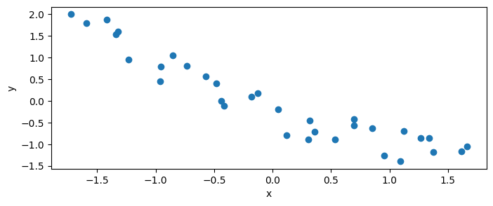
Cell 1.3: Fitting the linear model
Goal:
- Fit a linear model on the standardized data, as the baseline the quadratic model in Cell 1.4 will be compared against
Implementation:
mu = alpha + beta*x;idata_kwargs={"log_likelihood": True}is needed to later compute WAIC/LOO in Part 4
with pm.Model() as model_l:
    # mu = alpha + beta * x
    alpha = pm.Normal("alpha", mu=0, sigma=1)
    beta = pm.Normal("beta", mu=0, sigma=10)
    mu = alpha + beta * x_c[0]
    #
    sigma = pm.HalfNormal("sigma", 5)
    #
    y_pred = pm.Normal("y_pred", mu=mu, sigma=sigma, observed=y_c)
    #
    idata_l = pm.sample(2000, idata_kwargs={"log_likelihood": True})
    idata_l = pm.sample_posterior_predictive(idata_l, extend_inferencedata=True)
Cell 1.4: Fitting the quadratic model
Goal:
- Fit a quadratic model on the same data, to compare against the linear fit
Implementation:
mu = alpha + beta_1*x + beta_2*x^2, withbetaa 2-dim vector
with pm.Model() as model_p:
    # mu = alpha + beta_1 * x + beta_2 * x^2
    alpha = pm.Normal("alpha", mu=0, sigma=1)
    # Beta is a 2-dim vector.
    beta = pm.Normal("beta", mu=0, sigma=10, shape=order)
    mu = alpha + pm.math.dot(beta, x_c)
    #
    sigma = pm.HalfNormal("sigma", 5)
    #
    y_pred = pm.Normal("y_pred", mu=mu, sigma=sigma, observed=y_c)
    #
    idata_q = pm.sample(2000, idata_kwargs={"log_likelihood": True})
    idata_q = pm.sample_posterior_predictive(idata_q, extend_inferencedata=True)
Cell 1.5: Computing the posterior mean estimates
Goal:
- Extract the posterior mean of each model’s parameters, to plug into the fitted-line formula in Cell 1.6
# Sample the x space uniformly with 100 samples.
x_new = np.linspace(x_c[0].min(), x_c[0].max(), 100)

# Posterior.
posterior_l = az.extract(idata_l)
posterior_p = az.extract(idata_q)

# Compute the mean posterior of the linear model.
alpha_l_post = posterior_l["alpha"].mean().item()
beta_l_post = posterior_l["beta"].mean().item()
print(
    f"linear model: alpha_l_post={alpha_l_post:.2g}, "
    f"beta_l_post={beta_l_post:.2g}"
)

# Compute the mean posterior of the quadratic model.
alpha_p_post = posterior_p["alpha"].mean().item()
beta_p_post = posterior_p["beta"].mean("sample")
print(
    f"quadratic model: alpha_p_post={alpha_p_post:.2g}, "
    f"beta_post[0]={beta_p_post[0]:.2g}, beta_post[1]={beta_p_post[1]:.2g}"
)
Cell 1.6: Visualizing the fitted models
Goal:
- Plot the data together with the linear and quadratic mean-posterior fits, to see how much the extra quadratic term changes the fit
y_l_post = alpha_l_post + beta_l_post * x_new
plt.plot(x_new, y_l_post, "C0", label="linear model")

y_p_post = alpha_p_post + np.dot(beta_p_post, x_c)
plt.plot(x_c[0], y_p_post, "C1", label="quadratic model")

# Plot data.
plt.plot(x_c[0], y_c, "C2.")
plt.legend()
ut.save_plt("Lesson07.Comparing_models.model_fit.png")
Cell 1.7: Posterior predictive checks
Goal:
- Compare each model’s posterior-predictive distribution against the observed data
az.plot_ppc(idata_l, num_pp_samples=100, colors=["C1", "C0", "C1"])
plt.title("linear model")
ut.save_plt("Lesson07.Comparing_models.lin_model_PPC.png")
az.plot_ppc(idata_q, num_pp_samples=100, colors=["C1", "C0", "C1"])
plt.title("quadratic model")
ut.save_plt("Lesson07.Comparing_models.quadr_model_PPC.png")Part 2: Bayesian P-value
Cell 2.1: Comparing Bayesian p-value for mean and IQR
Goal:
- Compare the Bayesian p-value of the mean, and of the interquartile range, between the linear and quadratic models
Implementation: putils.iqr(x, a=-1)
- Interquartile range statistic, passed to
az.plot_bpv(t_stat=...)
colors = ["C0", "C1"]
idatas = [idata_l, idata_q]

_, axes = plt.subplots(1, 2)

# Plot the Bayesian p-value for mean for both models.
for idata, c in zip(idatas, colors):
    az.plot_bpv(idata, kind="t_stat", t_stat="mean", ax=axes[0], color=c)
axes[0].set_title("mean")

# Plot the Bayesian p-value for interquartile range for both models.
for idata, c in zip(idatas, colors):
    az.plot_bpv(idata, kind="t_stat", t_stat=putils.iqr, ax=axes[1], color=c)
axes[1].set_title("IQR")
Cell 2.2: Comparing Bayesian p-value for the entire distribution
Goal:
- Compare the Bayesian p-value computed over the entire distribution, rather than a single statistic
_, ax = plt.subplots()

for idata, c in zip(idatas, colors):
    az.plot_bpv(idata, color=c, ax=ax)
Part 3: Overfitting
Cell 3.1: In-sample vs out-of-sample data
Goal:
- Look at the in-sample data (black) plus 2 extra held-out points (red), used next to show how model order affects generalization
x0 = np.array([4.0, 5.0, 6.0, 9.0, 12, 14.0])
y0 = np.array([4.2, 6.1, 5.0, 10.0, 10, 14.0])
x1 = np.array([6.5, 10])
y1 = np.array([7, 10])

_, ax = plt.subplots(1, 1)
ax.plot(x0, y0, "ko")
ax.plot(x1, y1, "rs")
Cell 3.2: Fitting models of increasing order on in-sample data
Goal:
- Fit polynomials of order 0, 1, and 5 on the in-sample data, and check their R^2 on that same data
Implementation: putils.plot_models(x0, y0, ps, ax)
- Plots each fitted polynomial with its R^2 computed against
(x0, y0)
_, ax = plt.subplots(1, 1)
ax.plot(x0, y0, "ko", zorder=3)

# Learn 3 models.
order = [0, 1, 5]
ps = []
for i in order:
    p = np.polynomial.Polynomial.fit(x0, y0, deg=i)
    ps.append(p)

putils.plot_models(x0, y0, ps, ax)
Cell 3.3: Evaluating the fit models on out-of-sample data
Goal:
- Recompute each model’s R^2 including the 2 held-out points: the order-5 model’s R^2 collapses, showing it overfit the in-sample data
_, ax = plt.subplots(figsize=(12, 4))

ax.plot(x0, y0, "ko", zorder=3)
ax.plot(x1, y1, "rs", zorder=3)

x_all = np.concatenate((x0, x1))
y_all = np.concatenate((y0, y1))
putils.plot_models(x_all, y_all, ps, ax)
Part 4: Calculating Predictive Accuracy
Cell 4.1: WAIC
Goal:
- Compute the Widely Applicable Information Criterion for both models, an estimate of out-of-sample predictive accuracy
waic_l = az.waic(idata_l)
display(waic_l)
waic_q = az.waic(idata_q)
display(waic_q)Cell 4.2: LOO
Goal:
- Compute the Pareto-smoothed importance-sampling leave-one-out estimate for both models, an alternative to WAIC
loo_l = az.loo(idata_l)
display(loo_l)
loo_q = az.loo(idata_q)
display(loo_q)Part 5: Comparing Models
Cell 5.1: Model comparison table and plot
Goal:
- Rank the linear and quadratic models by predictive accuracy, using
az.compare()'s default (LOO-based) criterion
cmp_df = az.compare({"model_l": idata_l, "model_q": idata_q})
display(cmp_df)az.plot_compare(cmp_df)Part 6: Model Averaging
Cell 6.1: Weighted predictions
Goal:
- Combine both models’ posterior-predictive samples into a single weighted mixture, using pseudo-BMA-style weights
idatas = [idata_l, idata_q]
weights = [0.35, 0.65]
idata_w = az.weight_predictions(idatas, weights)
Cell 6.2: Visualizing the weighted posterior predictive
Goal:
- Compare the linear, quadratic, and weighted posterior-predictive densities on one plot
_, ax = plt.subplots(figsize=(10, 6))

# Linear.
az.plot_kde(
    idata_l.posterior_predictive["y_pred"].values,
    plot_kwargs={"color": "C0", "lw": 3},
    label="linear",
    ax=ax,
)

# Quadratic.
az.plot_kde(
    idata_q.posterior_predictive["y_pred"].values,
    plot_kwargs={"color": "C1", "lw": 3},
    label="quadratic",
    ax=ax,
)

# Weighted.
az.plot_kde(
    idata_w.posterior_predictive["y_pred"].values,
    plot_kwargs={"color": "C2", "lw": 3, "ls": "--"},
    label="weighted",
    ax=ax,
)

plt.legend()