Imports
%load_ext autoreload
%autoreload 2

!sudo /bin/bash -c "(source /venv/bin/activate; pip install --quiet graphviz)"
!sudo /bin/bash -c "(source /venv/bin/activate; pip install --quiet dataframe_image)"

import arviz as az
import pandas as pd
import xarray as xr
import pymc as pm
import numpy as np
import seaborn as sns
import matplotlib.pyplot as plt
from IPython.display import display
import helpers.htutorial as ut
import L07_04_generalized_linear_models_utils as putils
ut.config_notebook()
dir_name = "./L07_data"
!ls $dir_namePart 1: Linear Regression
Cell 1.1: Synthetic example
Goal:
- Fit a Bayesian linear regression on synthetic data with a known
alpha/beta/noise, so the recovered posterior can be checked against the ground truth
Implementation:
alpha ~ Normal(0, 10),beta ~ Normal(0, 1),sigma ~ HalfCauchy(5),y ~ Normal(alpha + beta*x, sigma)
np.random.seed(1)

# Number of samples.
N = 100

# Ground-truth parameters.
alpha_real = 2.5
beta_real = 0.9
sigma_eps_real = 0.5

# Generate data.
x = np.random.normal(10, 1, N)
y_real = alpha_real + beta_real * x

# Add noise.
eps_real = np.random.normal(0, sigma_eps_real, size=N)
y = y_real + eps_real
sns.scatterplot(x=x, y=y_real, label="noiseless")
sns.scatterplot(x=x, y=y, label="observed")df = pd.DataFrame({"X": x, "Y": y})
sns.regplot(
x="X",
y="Y",
data=df,
scatter_kws={"color": "blue"},
line_kws={"color": "red"},
)<Axes: xlabel='X', ylabel='Y'>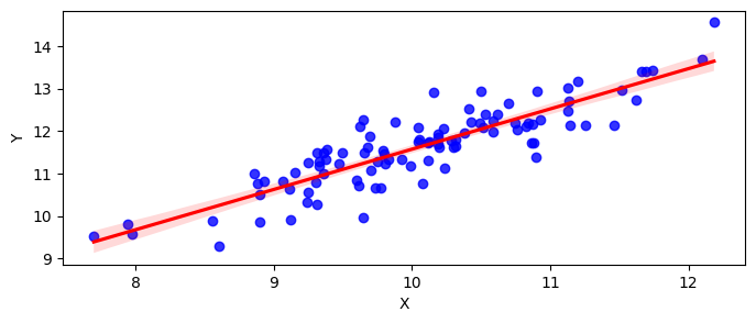
with pm.Model() as model_g:
    # Priors, wide relative to the ground-truth values above.
    alpha = pm.Normal("alpha", mu=0, sigma=10)
    beta = pm.Normal("beta", mu=0, sigma=1)
    sigma = pm.HalfCauchy("sigma", 5)
    # Linear predictor and Normal likelihood.
    mu = pm.Deterministic("mu", alpha + beta * x)
    y_pred = pm.Normal("y_pred", mu=mu, sigma=sigma, observed=y)
    idata_g = pm.sample(2000, tune=1000)
Auto-assigning NUTS sampler...
Initializing NUTS using jitter+adapt_diag...
Multiprocess sampling (4 chains in 4 jobs)
NUTS: [alpha, beta, sigma]
Loading...
Loading...
Sampling 4 chains for 1_000 tune and 2_000 draw iterations (4_000 + 8_000 draws total) took 6 seconds.
pm.model_to_graphviz(model_g)Loading...
az.plot_trace(idata_g, var_names=["alpha", "beta", "sigma"])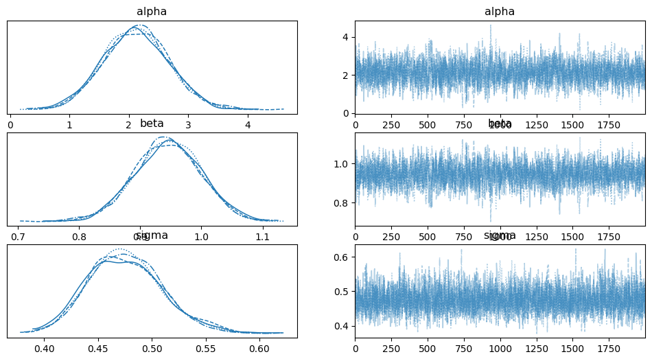
display(az.summary(idata_g, var_names="alpha beta sigma".split(), kind="stats"))Loading...
Cell 1.2: Bike rental example
Goal:
- Fit the same linear-regression pattern to real data: predicting bike rentals from temperature
Implementation:
- Same
alpha/beta/sigmapriors asmodel_g, refit onbikes.temperature/bikes.rented putils.plot_data_and_model()overlays the fitted mean and 50%/94% posterior-predictive bands on the raw data
bikes = pd.read_csv(dir_name + "/bikes.csv")
bikes.plot(x="temperature", y="rented", figsize=(12, 3), kind="scatter")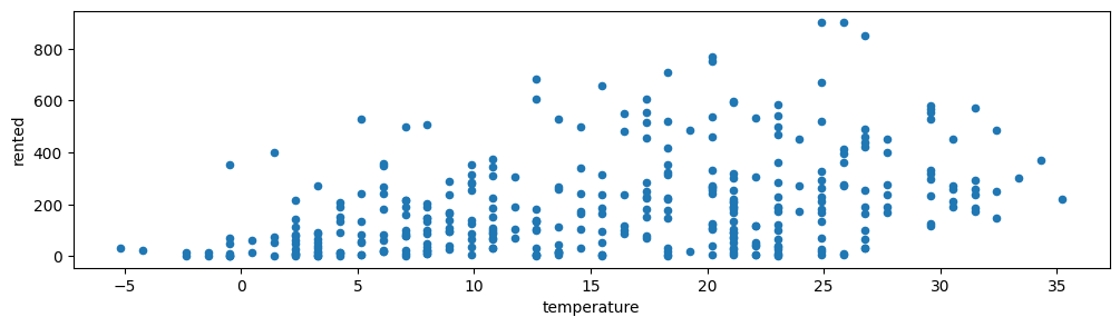
display(bikes.head())Loading...
with pm.Model() as model_lb:
    alpha = pm.Normal("alpha", mu=0, sigma=100)
    beta = pm.Normal("beta", mu=0, sigma=10)
    sigma = pm.HalfCauchy("sigma", 10)
    # Linear predictor and Normal likelihood.
    mu = pm.Deterministic("mu", alpha + beta * bikes.temperature)
    y_pred = pm.Normal("y_pred", mu=mu, sigma=sigma, observed=bikes.rented)
    idata_lb = pm.sample()
Auto-assigning NUTS sampler...
Initializing NUTS using jitter+adapt_diag...
Multiprocess sampling (4 chains in 4 jobs)
NUTS: [alpha, beta, sigma]
Loading...
Loading...
Sampling 4 chains for 1_000 tune and 1_000 draw iterations (4_000 + 4_000 draws total) took 2 seconds.
# Plot all the vars, excluding mu.
az.plot_posterior(idata_lb, var_names=["~mu"])
# Sample from the posterior.
posterior = az.extract(idata_lb, num_samples=50)

# Create 50 equally-spaced points from min to max temperature.
x_plot = xr.DataArray(
    np.linspace(bikes.temperature.min(), bikes.temperature.max(), 50),
    dims="plot_id",
)
# Compute the expected value of the model for these points.
mean_line = posterior["alpha"].mean() + posterior["beta"].mean() * x_plot
# Compute 50 lines using the posterior.
lines = posterior["alpha"] + posterior["beta"] * x_plot
print("x_plot.shape=", x_plot.shape)
print("mean_line.shape=", mean_line.shape)
idata_lb_pp = pm.sample_posterior_predictive(idata_lb, model=model_lb)
mean_line = idata_lb.posterior["mu"].mean(("chain", "draw"))# Plot the data.
# zorder is to plot behind the line.
plt.plot(bikes.temperature, bikes.rented, "C2.", zorder=-3)
# Plot the 50 models from the posterior.
# lines.T.values are the 50 lines.
lines_ = plt.plot(x_plot, lines.T.values, c="C1", alpha=0.2, label="lines")
# Remove the label for all the lines but the first one.
plt.setp(lines_[1:], label="_")
plt.xlabel("temp")
plt.ylabel("rented bikes")
_ = plt.legend()Sampling: [y_pred]
Loading...
Loading...
putils.plot_data_and_model(bikes, idata_lb_pp, mean_line)(50,)
Part 2: Counting
Cell 2.1: Fitting a Negative Binomial model
Goal:
- Refit the bike-rental data with a Negative Binomial likelihood, better suited to non-negative counts than the Gaussian model in Part 1
Implementation:
mu = exp(alpha + beta*temperature)keeps the mean positive;y ~ NegativeBinomial(mu, sigma), wheresigmacontrols the variance
np.random.seed(42)
with pm.Model() as model_neg:
    alpha = pm.Normal("alpha", mu=0, sigma=100)
    beta = pm.Normal("beta", mu=0, sigma=10)
    # We use exp to keep the mean positive.
    mu = pm.Deterministic("mu", pm.math.exp(alpha + beta * bikes.temperature))
    # NegativeBinomial has an extra param, sigma, to control the variance.
    sigma = pm.HalfNormal("sigma", 10)
    y_pred = pm.NegativeBinomial(
        "y_pred", mu=mu, alpha=sigma, observed=bikes.rented
    )
    #
    idata_neg = pm.sample()
    idata_neg = pm.sample_posterior_predictive(
        idata_neg, extend_inferencedata=True
    )
(348,)
pm.model_to_graphviz(model_neg)Loading...
az.plot_trace(idata_neg, var_names=["~mu"])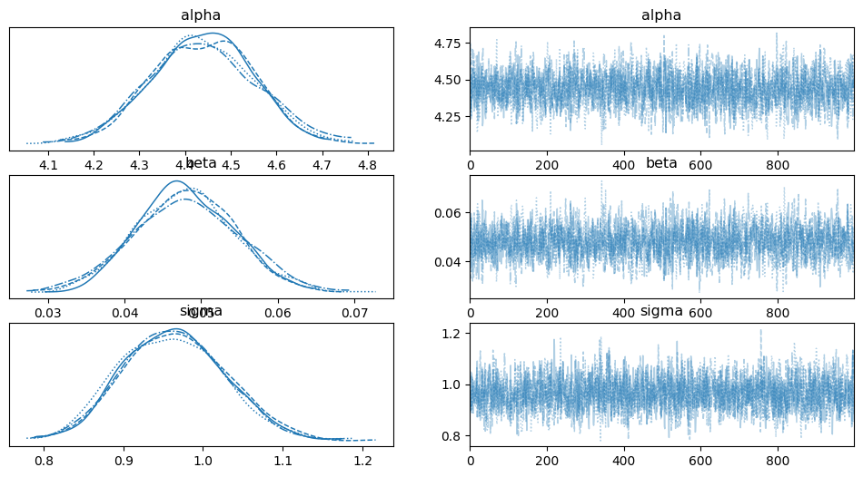
Cell 2.2: Comparing posterior predictive checks
Goal:
- Compare the Negative Binomial fit against the Gaussian fit from Part 1, on both the fitted curve and the posterior-predictive distribution
putils.plot_data_and_model(bikes, idata_neg, mean_line)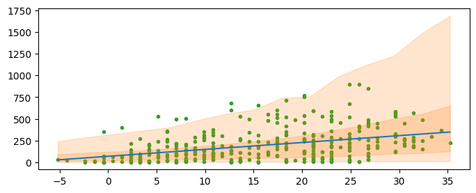
az.plot_ppc(idata_lb_pp, num_pp_samples=200, alpha=0.1, mean=False)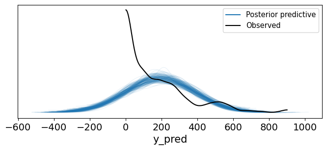
az.plot_ppc(idata_neg, num_pp_samples=200, alpha=0.1, mean=False)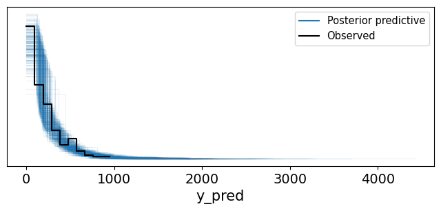
Part 3: Robust Regression
Cell 3.1: Anscombe’s outlier dataset
Goal:
- Look at a small dataset with one clear outlier, used next to contrast a non-robust and a robust regression
ans = pd.read_csv(dir_name + "/anscombe_3.csv")
display(ans.head())
Loading...
ans.plot("x", "y", kind="scatter")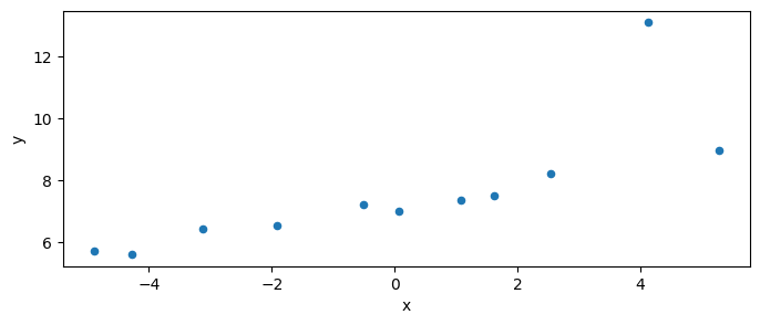
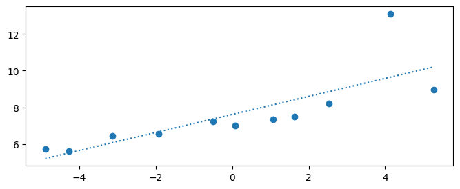
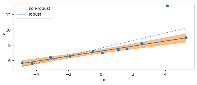
Cell 3.2: Non-robust vs robust fit
Goal:
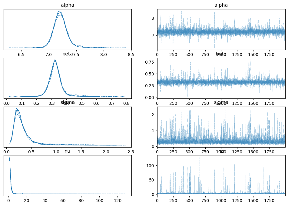
- Fit an ordinary least-squares line (sensitive to the outlier) and a Bayesian Student-t regression (robust to it), and compare both fits
Implementation:
- OLS via
scipy.stats.linregress - Student-t model:
nu ~ Exponential(1/29) + 1(shifted sonu >= 1),y ~ StudentT(alpha + beta*x, sigma, nu)
import scipy

beta_c, alpha_c, *_ = scipy.stats.linregress(ans.x, ans.y)

_, ax = plt.subplots()
ax.plot(ans.x, (alpha_c + beta_c * ans.x), "C0:", label="non-robust")
ax.plot(ans.x, ans.y, "C0o")
ut.save_ax(ax, "Lesson07_Non_robust_regression1.png")
with pm.Model() as model_t:
    # Alpha is Normal, centered around the mean of the y data.
    alpha = pm.Normal("alpha", mu=ans.y.mean(), sigma=1)
    # Beta is standard Normal(0, 1).
    beta = pm.Normal("beta", mu=0, sigma=1)
    sigma = pm.HalfNormal("sigma", 5)
    # The Exponential puts too much weight close to 0, so shift by 1.
    nu_ = pm.Exponential("nu_", 1 / 29)
    nu = pm.Deterministic("nu", nu_ + 1)

    # Linear predictor and Student-t likelihood.
    mu = pm.Deterministic("mu", alpha + beta * ans.x)
    y_pred = pm.StudentT("y_pred", mu=mu, sigma=sigma, nu=nu, observed=ans.y)
    idata_t = pm.sample(2000, tune=2000)
    idata_t = pm.sample_posterior_predictive(idata_t, extend_inferencedata=True)
Auto-assigning NUTS sampler...
Initializing NUTS using jitter+adapt_diag...
Multiprocess sampling (4 chains in 4 jobs)
NUTS: [alpha, beta, sigma, nu_]
Loading...
Loading...
Sampling 4 chains for 2_000 tune and 2_000 draw iterations (8_000 + 8_000 draws total) took 3 seconds.
Sampling: [y_pred]
Loading...
Loading...
ut.save_dot(model_t, "Lesson07_Robust_regression_model")
var_names = "alpha beta sigma nu".split()
az.plot_trace(idata_t, var_names=var_names)
display(az.summary(idata_t, var_names=var_names, round_to=2, kind="stats"))
Loading...
_, ax = plt.subplots()

# Non-robust.
ax.plot(ans.x, (alpha_c + beta_c * ans.x), "C0:", label="non-robust")
ax.plot(ans.x, ans.y, "C0o")

# Robust.
alpha_m = idata_t.posterior["alpha"].mean(("chain", "draw"))
beta_m = idata_t.posterior["beta"].mean(("chain", "draw"))

x_plot = xr.DataArray(np.linspace(ans.x.min(), ans.x.max(), 50), dims="plot_id")
ax.plot(x_plot, alpha_m + beta_m * x_plot, c="C0", label="robust")
az.plot_hdi(ans.x, az.hdi(idata_t.posterior["mu"])["mu"].T, ax=ax)
ax.set_xlabel("x")
ax.set_ylabel("y", rotation=0)
ax.legend(loc=2)
ut.save_ax(ax, "Lesson07_Non_robust_regression2")
/venv/lib/python3.12/site-packages/arviz/plots/hdiplot.py:166: FutureWarning: hdi currently interprets 2d data as (draw, shape) but this will change in a future release to (chain, draw) for coherence with other functions
  hdi_data = hdi(y, hdi_prob=hdi_prob, circular=circular, multimodal=False, **hdi_kwargs)
Cell 3.3: Posterior predictive check
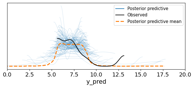
Goal:
- Check the robust model’s posterior-predictive fit against the data
# Posterior predictive check.
ppc = pm.sample_posterior_predictive(
    idata_t,
    model=model_t,
    random_seed=2,
)
az.plot_ppc(idata_t, mean=True, num_pp_samples=100)
plt.xlim(0, 20)
Part 4: Logistic Regression
Cell 4.1: Iris data for two species
Goal:
- Prepare a 2-class subset of the iris dataset and one feature, sepal
length, to classify
setosavsversicolor
iris = pd.read_csv(dir_name + "/iris.csv")
display(iris.head())
ut.save_df(iris.head(), "Lesson07_Logistic_regression_df.png")
Sampling: [y_pred]
Loading...
Loading...
# Filter the dataframe keeping only 2 values for species.
df = iris.query("species == ('setosa', 'versicolor')")
display(df.head())
# Get the predicted variable.
y_0 = pd.Categorical(df["species"]).codes
print("y_0=", y_0)# Get the sepal length as feature, centered.
x_n = "sepal_length"
x_0 = df[x_n].values
x_c = x_0 - x_0.mean()Cell 4.2: Fitting a logistic regression
Goal:
- Fit a Bayesian logistic regression, and derive the decision boundary
bdwhere the predicted probability crosses 0.5
Implementation:
theta = sigmoid(alpha + beta*x_c),y ~ Bernoulli(theta);bd = -alpha / betais the boundary wheretheta = 0.5
with pm.Model() as model_lrs:
    # Linear part.
    alpha = pm.Normal("alpha", mu=0, sigma=1)
    beta = pm.Normal("beta", mu=0, sigma=5)
    mu = alpha + x_c * beta
    # Sigmoid link.
    theta = pm.Deterministic("theta", pm.math.sigmoid(mu))
    # Likelihood.
    yl = pm.Bernoulli("yl", p=theta, observed=y_0)
    # Decision boundary: theta = 0.5.
    bd = pm.Deterministic("bd", -alpha / beta)
    #
    idata_lrs = pm.sample(random_seed=123)
Loading...
ut.save_dot(model_lrs, "Lesson07_Logistic_regression_model.png")
var_names = ["~bd", "~theta"]
display(az.summary(idata_lrs, var_names=var_names, round_to=2, kind="stats"))
Loading...
ax = az.plot_trace(idata_lrs, var_names=var_names)
ut.save_fig(ax, "Lesson07_Logistic_regression_result.png")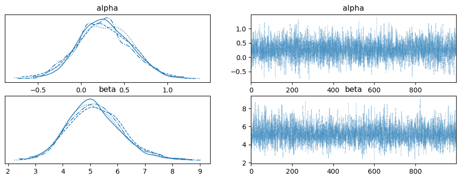
Cell 4.3: Visualizing the decision boundary
Goal:
- Plot the fitted sigmoid, the decision boundary and its HDI, and the raw data together
posterior = idata_lrs.posterior
theta = posterior["theta"].mean(("chain", "draw"))
idx = np.argsort(x_c)

# Plot the model.
_, ax = plt.subplots()
ax.plot(x_c[idx], theta[idx], color="C0", lw=2)

# Plot the decision boundary and its HDI.
ax.vlines(posterior["bd"].mean(("chain", "draw")), 0, 1, color="C2", zorder=0)
bd_hdi = az.hdi(posterior["bd"])
ax.fill_betweenx(
    [0, 1], bd_hdi["bd"][0], bd_hdi["bd"][1], color="C2", alpha=0.6, lw=0
)

# Plot the data.
ax.scatter(x_c, np.random.normal(y_0, 0.02), marker=".")
az.plot_hdi(x_c, posterior["theta"], color="C0", ax=ax)
ut.save_ax(ax, "Lesson07_Logistic_regression_result2.png")
Part 5: Variable Variance
Cell 5.1: Babies growth data
Goal:
- Look at babies’ length by age in months: the spread grows with age, so a constant-variance model would be a poor fit
data = pd.read_csv(dir_name + "/babies.csv")
data.columns = ["month", "length"]
data.plot.scatter("month", "length")
display(data.head())
Loading...
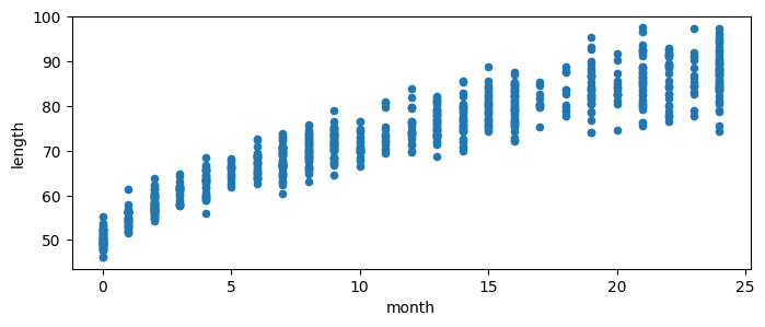
ax = data.plot.scatter("month", "length")
ut.save_ax(ax, "Lesson07_Variable_variance_data.png")
Cell 5.2: Fitting a model with variance as a function of age
Goal:
- Model both the mean and the standard deviation as functions of
month, instead of assuming constant variance
Implementation:
mu = alpha + beta*sqrt(month),sigma = gamma + delta*month,y ~ Normal(mu, sigma)
with pm.Model() as model_vv:
    # Create a shared variable so the data can change after the model is built.
    x_shared = pm.Data("x_shared", data.month.values.astype(float))
    # Linear model for the mean is a function of sqrt(month).
    alpha = pm.Normal("alpha", sigma=10)
    beta = pm.Normal("beta", sigma=10)
    mu = pm.Deterministic("mu", alpha + beta * x_shared**0.5)
    # Linear model for the std dev.
    gamma = pm.HalfNormal("gamma", sigma=10)
    delta = pm.HalfNormal("delta", sigma=10)
    sigma = pm.Deterministic("sigma", gamma + delta * x_shared)
    # Fit.
    y_pred = pm.Normal("y_pred", mu=mu, sigma=sigma, observed=data.length)
    #
    idata_vv = pm.sample(random_seed=123)
Auto-assigning NUTS sampler...
Initializing NUTS using jitter+adapt_diag...
Multiprocess sampling (4 chains in 4 jobs)
NUTS: [alpha, beta, gamma, delta]
Loading...
Loading...
Sampling 4 chains for 1_000 tune and 1_000 draw iterations (4_000 + 4_000 draws total) took 2 seconds.
pm.model_to_graphviz(model_vv)
ut.save_dot(model_vv, "Lesson07_Variable_variance_model.png")
Loading...
Cell 5.3: Visualizing the fitted mean and variance bands
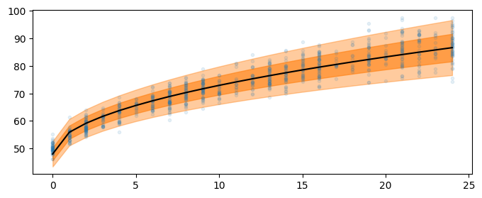
Goal:
- Plot the fitted mean with 1 and 2 standard-deviation bands against the raw data, to see the variance growing with age
# Plot the data.
plt.plot(data.month, data.length, "C0.", alpha=0.1)

# Compute the posterior mean and sigma.
posterior = az.extract(idata_vv)
mu_m = posterior["mu"].mean("sample").values
sigma_m = posterior["sigma"].mean("sample").values

# Plot 1 and 2 std dev of the model.
plt.plot(data.month, mu_m, c="k")
plt.fill_between(
    data.month, mu_m + 1 * sigma_m, mu_m - 1 * sigma_m, alpha=0.6, color="C1"
)
plt.fill_between(
    data.month, mu_m + 2 * sigma_m, mu_m - 2 * sigma_m, alpha=0.4, color="C1"
)
ut.save_plt("Lesson07_Variable_variance_result.png")
Part 6: Multiple Linear Regression
Cell 6.1: Synthetic multi-feature data
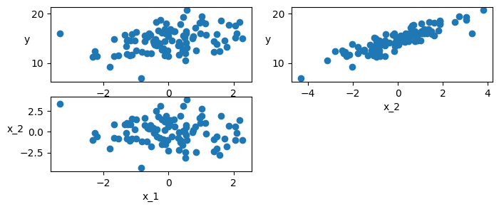
Goal:
- Generate synthetic data with 2 independent features, to fit a multiple linear regression against a known ground truth
Implementation: putils.scatter_plot(x, y)
- Plots
yagainst each feature, plus the two features against each other, in a 1xN layout
np.random.seed(314)

N = 100
alpha_real = 2.5
beta_real = [0.9, 1.5]
eps_stddev_real = 0.5
eps_real = np.random.normal(0, eps_stddev_real, size=N)

# Independent variables, means [10, 2] and std devs [1, 1.5].
X = np.array([np.random.normal(i, j, N) for i, j in zip([10, 2], [1, 1.5])]).T
X_mean = X.mean(axis=0, keepdims=True)
X_centered = X - X_mean

# Create samples.
y = alpha_real + np.dot(X, beta_real) + eps_real
putils.scatter_plot(X_centered, y)
ut.save_plt("Lesson07_Multiple_linear_regression3.png")
Cell 6.2: Fitting the multiple regression model
Goal:
- Fit the multiple linear regression, centering
Xfor a more stable sampler geometry, then recovering the original-scale intercept
Implementation:
alpha_tmp ~ Normal(0, 10),beta ~ Normal(0, 1)(length 2), fit onX_centered;alpha = alpha_tmp - X_mean . betaundoes the centering
with pm.Model() as model_mlr:
    alpha_tmp = pm.Normal("alpha_tmp", mu=0, sigma=10)
    # Beta is a length-2 vector, one weight per feature.
    beta = pm.Normal("beta", mu=0, sigma=1, shape=2)
    eps = pm.HalfCauchy("eps", 5)
    # Linear predictor on the centered features.
    mu = alpha_tmp + pm.math.dot(X_centered, beta)
    # Recover the original-scale intercept.
    alpha = pm.Deterministic("alpha", alpha_tmp - pm.math.dot(X_mean, beta))

    # Likelihood.
    y_pred = pm.Normal("y_pred", mu=mu, sigma=eps, observed=y)
    idata_mlr = pm.sample(2000)
Auto-assigning NUTS sampler...
Initializing NUTS using jitter+adapt_diag...
Multiprocess sampling (4 chains in 4 jobs)
NUTS: [alpha_tmp, beta, eps]
Loading...
Loading...
Sampling 4 chains for 1_000 tune and 2_000 draw iterations (4_000 + 8_000 draws total) took 2 seconds.
ut.save_dot(model_mlr, "Lesson07_Multiple_linear_regression_model.png")
pm.model_to_graphviz(model_mlr)
Loading...
Cell 6.3: Inspecting the fit
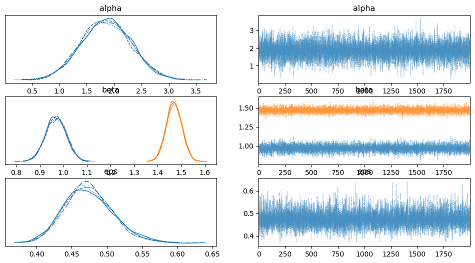
Goal:
- Check the sampling trace and numerical summary against the known
ground-truth
alpha_real/beta_real
var_names = ["alpha", "beta", "eps"]
az.plot_trace(idata_mlr, var_names=var_names)
ut.save_plt("Lesson07_Multiple_linear_regression_results1.png")
mlr_summary = az.summary(
    idata_mlr, var_names=var_names, round_to=2, kind="stats"
)
ut.save_df(mlr_summary, "Lesson07_Multiple_linear_regression_results2.png")
display(mlr_summary)
Loading...
Part 7: Rented Bikes With Two Predictors
Cell 7.1: Fitting a Negative Binomial model with two predictors
Goal:
- Extend Part 2’s single-predictor Negative Binomial model with a second
predictor,
hour, to see if it improves the fit
Implementation:
mu = exp(alpha + beta0*temperature + beta1*hour),y ~ NegativeBinomial(mu, sigma)
with pm.Model() as model_mlb:
    alpha = pm.Normal("alpha", mu=0, sigma=1)
    beta0 = pm.Normal("beta0", mu=0, sigma=10)
    beta1 = pm.Normal("beta1", mu=0, sigma=10)
    sigma = pm.HalfNormal("sigma", 10)
    mu = pm.Deterministic(
        "mu", pm.math.exp(alpha + beta0 * bikes.temperature + beta1 * bikes.hour)
    )
    _ = pm.NegativeBinomial("y_pred", mu=mu, alpha=sigma, observed=bikes.rented)
    #
    idata_mlb = pm.sample()
Auto-assigning NUTS sampler...
Initializing NUTS using jitter+adapt_diag...
Multiprocess sampling (4 chains in 4 jobs)
NUTS: [alpha, beta0, beta1, sigma]
Loading...
Loading...
Sampling 4 chains for 1_000 tune and 1_000 draw iterations (4_000 + 4_000 draws total) took 2 seconds.
pm.model_to_graphviz(model_mlb)
ut.save_dot(
    model_mlb, "Lesson07_Multiple_linear_regression_model_RentedBikes_model.png"
)
Loading...
Cell 7.2: Inspecting the fit
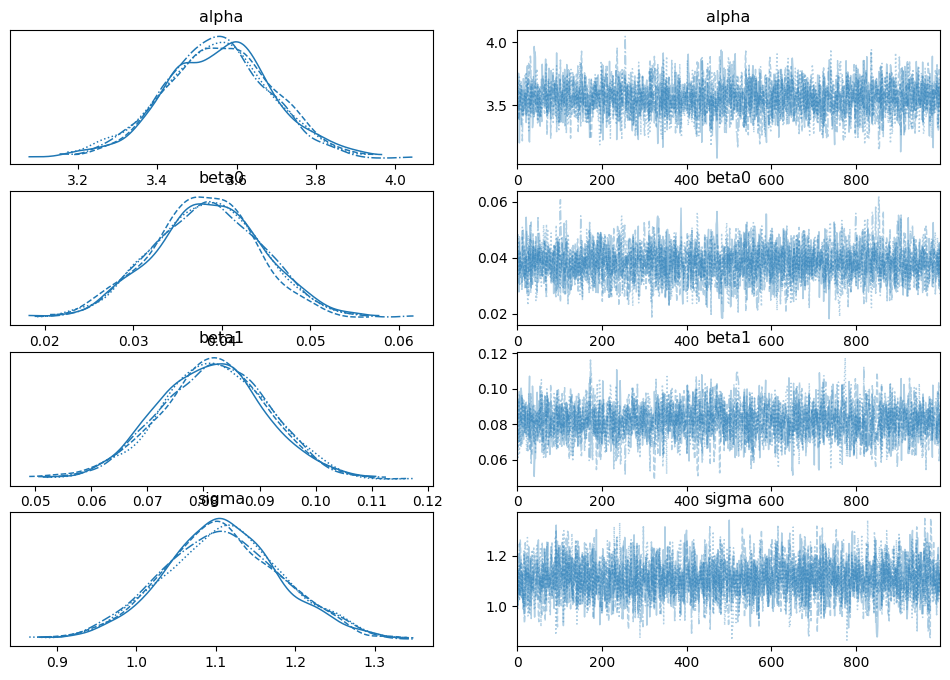
Goal:
- Check the sampling trace and numerical summary for the two-predictor model
var_names = ["alpha", "beta0", "beta1", "sigma"]
az.plot_trace(idata_mlb, var_names=var_names)
ut.save_plt(
    "Lesson07_Multiple_linear_regression_model_RentedBikes_model_trace.png"
)
mlb_summary = az.summary(
    idata_mlb, var_names=var_names, round_to=2, kind="stats"
)
display(mlb_summary)
Loading...