Table of Contents

!conda info --envs

import functools

import numpy as np
import matplotlib.pyplot as plt
import pandas as pd

%matplotlib inline

import notebook_utils

notebook_utils.notebook_config()
# matplotlib.rcParams["figure.figsize"] = (15, 6)

# assert np.__version__ == "1.33.3"
assert pd.__version__ == "0.20.3"
# assert matplotlib.__version__ == "2.0.2"

from notebook_utils import display_df

from IPython.display import display

# def display_df(df):
#     display(df)

# .loc[] vs .ix[] vs .iloc[]

# .ix supports mixed integer and label based access
# It is primarily label based, but will fall back to integer positional access unless the
# corresponding axis is of integer type.
# .ix is the most general and will support any of the inputs in .loc and .iloc.
# .ix also supports floating point label schemes.
# .ix is exceptionally useful when dealing with mixed positional and label based hierachical indexes.

# When an axis is integer based, ONLY label based access and not positional access is supported.
# Thus, in such cases, it’s usually better to be explicit and use .iloc or .loc.

# TODO: Add examples.

df = pd.DataFrame(
    [[1, 2, 0], [3, 4, 0], [5, 6, 0]],
    index="a b c".split(),
    columns="A B C".split(),
)
df

df.xs("a", axis=0)

df.xs("A", axis=1)

df.xs(["A", "B"], axis=1)

# ?
df.xs(slice("A", "C"), axis=1)

df.loc["a"]

df["A"]

df.iloc[0]

df_orig = pd.DataFrame(
    {"AAA": [4, 5, 6, 7], "BBB": [10, 20, 30, 40], "CCC": [100, 50, -30, -50]}
)

# These are equivalent syntax.
print(df_orig["AAA"])

print(df_orig.AAA)

df = df_orig.copy()
df

# Select a piece of the df and overwrite part of it.
# .ix[] is the same as .loc[]
df.ix[df.AAA >= 5, "BBB"] = -1
df

# Select a piece of the df and overwrite part of it.
df.loc[df.AAA >= 5, "BBB"] = -1
df

# Select a piece of df and overwrite it.
df.ix[df.AAA >= 5, ["BBB", "CCC"]] = 555
df

# Selecting a df through a mask.
df = df_orig.copy()
mask = pd.DataFrame(
    {"AAA": [True] * 4, "BBB": [False] * 4, "CCC": [True, False] * 2}
)
mask

# Filter df using df.where() and a boolean mask.
# nan is returned where the mask is False, the value of the df
# where the mask is True.
df.where(mask)

# Return a different value for when the mask is False.
df.where(mask, other="high")

# Use np.where().

column = df.AAA
np.where(column, "high", "low")

# Select rows based on certain criteria.
df = df_orig.copy()

dflow = df[df.AAA <= 5]
dfhigh = df[df.AAA > 5]

print(dflow)
print(dfhigh)

mask = (df.BBB < 25) & (df.CCC >= -40)
df.loc[mask, "AAA"]

df.loc[mask, "AAA":"BBB"]

df[mask][["AAA", "BBB"]]

df.ix[(df.CCC - 43.0).abs().argsort()]

c1 = df.AAA <= 5.5
c2 = df.BBB == 10.0
c3 = df.CCC > -40.0
cs = [c1, c2, c3]

print(functools.reduce(lambda x, y: x & y, cs))

print(c1 & c2 & c3)

df.index.isin([0, 2, 4])

df = df_orig.copy()
df = pd.DataFrame(
    df.values, index=["foo", "bar", "boo", "kar"], columns=df.columns
)
df

df.loc["bar":"kar"]

df.ix[0:3]

df.iloc[0:3]

df = df_orig.copy()
df

# Select columns where the column-wise column is larger than 30.
col_mask = df.sum() > 30

df.loc[:, col_mask]

df = pd.DataFrame(
    {"AAA": [1, 1, 1, 2, 2, 2, 3, 3], "BBB": [2, 1, 3, 4, 5, 1, 2, 3]}
)

df

# Find index of the min of one column.
np.argmin(df["BBB"])

# Find rows where there is a minimum of df["BBB"].
mask = df["BBB"] == np.min(df["BBB"])
df[mask]

df = pd.DataFrame(
    {"AAA": [1, 2, 1, 3], "BBB": [1, 1, 2, 2], "CCC": [2, 1, 3, 1]}
)

df["CCC"].idxmin()

# groupby AAA values and find the min in BBB.
df.groupby("AAA")["BBB"].idxmin()

df.sort_values(by=["BBB", "CCC"])

mask = df["AAA"] == np.min(df["AAA"])
df[mask]

# Add new cols converting numbers into greek letters.
df = pd.DataFrame(
    {"AAA": [1, 2, 1, 3], "BBB": [1, 1, 2, 2], "CCC": [2, 1, 3, 1]}
)
print("before=\n", df.to_string())

source_cols = df.columns
new_cols = [str(x) + "_cat" for x in source_cols]
categories = {1: "Alpha", 2: "Beta", 3: "Charlie"}
df[new_cols] = df[source_cols].applymap(lambda x: categories[x])
print("after=\n", df.to_string())

# This df uses a _ to separate and encode conceptually the multi-index.
# Construct the df by columns.
df = pd.DataFrame(
    {
        "row": [0, 1, 2],
        "One_X": [1.1, 1.1, 1.1],
        "One_Y": [1.2, 1.2, 1.2],
        "Two_X": [1.11, 1.11, 1.11],
        "Two_Y": [1.22, 1.22, 1.22],
    }
)
df = df.set_index("row")
display_df(df)

# print "columns=", df.columns
# print "index=", df.index

# Split the columns into tuples.
new_cols = [c.split("_") for c in df.columns]
print("new_cols=", new_cols)
tuples = list(map(tuple, new_cols))
print("tuples=", tuples)

# Convert the columns into a multi-index.
midx = pd.MultiIndex.from_tuples(tuples)
print("midx=", midx)
df2 = df.copy()
df2.columns = midx

# Note that the multi-index is represented as a cartesian product of labels
# (each of them associated to an index for uniqueness).
display_df(df2)

# stack() moves a level of column multi-indexing to the index (i.e., pivot)
df3 = df2.stack(0)
# print "columns=", df3.columns
# print "index=", df3.index
df3.head()

# reset_index() converts a level of indexing into a column.
# Conceptually reset_index() is the opposite of set_index() using multiple columns.
df4 = df3.reset_index(1)

df4

df5 = df3.reset_index(0)

df5

# help(pd.DataFrame.stack)

df = pd.DataFrame([[1, 2], [3, 4]], index=["one", "two"], columns=["a", "b"])
df

# stack() moves the column index into rows getting a pd.Series.
srs = df.stack()
print("srs=\n", srs)

print("\nindex=\n", srs.index)

np.random.seed(42)
df = pd.DataFrame(np.random.randint(0, 10, (5, 3)), columns="a b c".split())

display(df)

tuples = [(x, y) for x in "A B C".split() for y in "O I".split()]
print("tuples=", tuples)

cols = pd.MultiIndex.from_tuples(tuples)
print("cols=", cols)

# To get the values of the multi-index columns.
cols.get_values()

# Build a df with the given multi-index as columns.
np.random.seed(1000)
df = pd.DataFrame(
    np.random.randn(2, len(cols.get_values())), index="n m".split(), columns=cols
)
df

# Broadcast each level.
df.div(df["C"], level=1)

coords = [
    ("AA", "one"),
    ("AA", "six"),
    ("BB", "one"),
    ("BB", "two"),
    ("BB", "six"),
]

# Use multi-index index.
index = pd.MultiIndex.from_tuples(coords)

df = pd.DataFrame([11, 22, 33, 44, 55], index, columns=["data"])
df

# Select a row with .loc
df.loc["BB"]

# Select a row with xs using innermost index.
df.xs("BB", level=0, axis=0)

# Select a row using outermost index.
df.xs("six", level=1, axis=0)

import itertools

# Build multi-index for index (using Cartesian product).
index = list(
    itertools.product(["Ada", "Quinn", "Violet"], ["Comp", "Math", "Sci"])
)
print("index=", index)

index = pd.MultiIndex.from_tuples(index, names=["Student", "Course"])
print("midx=", index)

# Build another multi-index for columns.
columns = list(itertools.product(["Exams", "Labs"], ["I", "II"]))
print("columns=", columns)

# Cols are not named.
cols = pd.MultiIndex.from_tuples(columns)
print("midx=", cols)

# Build df.
data = [
    [70 + x + y + (x * y) % 3 for x in range(len(cols))]
    for y in range(len(index))
]
df = pd.DataFrame(data, index, cols)
df

# Select one row.
df.loc["Violet"]

# Select various cubes.
all_ = slice(None)
df.loc[(all_, "Math"), all_]

df.loc[(slice("Ada", "Violet"), "Math"), all_]

df.loc[(all_, "Math"), ("Exams")]

df.loc[(all_, "Math"), (all_, "II")]

df

# Sort by last columns.
df.sort_values(by=("Labs", "II"), ascending=False)

np.random.seed(1000)
df = pd.DataFrame(
    {
        "A": "a1 a1 a2 a3".split(),
        "B": "b1 b2 b3 b4".split(),
        "Vals": np.random.rand(4),
    }
)
df

# Group by column "A" and sum.
df.groupby("A").sum()

# Split by two columns.
df.groupby("A B".split()).sum()

df["firstLevel"] = "foo"
df

df.set_index("firstLevel")

df2 = df.groupby("A B".split()).sum()
df2["firstLevel"] = "foo"
df2 = df2.set_index("firstLevel", append=True)

# reorder_levels() reorder the levels in an index.
df2.reorder_levels(["firstLevel", "A", "B"])

df = pd.DataFrame([[5, 6, 7], [0, 1, 2]], columns=list("abc"), index=list("12"))
df

df.applymap(lambda x: x + 1)

def reduce_(x):
    return sum(x)


display_df(df)
print(df.apply(reduce_, axis=0))
print(df.apply(reduce_, axis=1))

np.random.seed(1000)

index = "a c e f h".split()
print("index", index)

columns = "one two three".split()
print("cols", columns)

df = pd.DataFrame(np.random.randn(5, 3), index=index, columns=columns)
display_df(df)

# Add column.
df["four"] = "bar"
df

# Add column function of another column.
df["five"] = df["one"] > 0
df

# Add more indices by re-indexing.
df2 = df.reindex("a b c d e f g h".split())
df2

df2["one"].isnull()

df2["one"].notnull()

df2.empty

df2.isnull()

print("None == None:", None == None)
print("np.nan == np.nan:", np.nan == np.nan)

# Can't check for nan-ness by comparison.
# Need to use isnull() or np.isnan().
df2["one"] == np.nan

df2["timestamp"] = pd.Timestamp("20120101")
display_df(df2)
print(df.dtypes)

pd.Timestamp("2012-01-01 05:00", tz="EST")

# Setting a nan automatically get converted in the proper value depending on the
# column type.
df2.ix[["a", "c", "h"], ["one", "timestamp"]] = np.nan
display_df(df2)
print(df2.dtypes)

print("pd.NaT == np.nan:", pd.NaT == np.nan)
print("pd.isnull(pd.NaT):", pd.isnull(pd.NaT))

print(df2.dtypes)

print(df2.get_dtype_counts())

s = pd.Series([1, 2, 3])
print(s)

# Since it is a container for floats None -> nan.
s.loc[0] = None
print(s)

s = pd.Series([1, 2, 3])
print(s)
# writing a char forces a type conversion of the container
s.loc[0] = "a"
print(s)

s = pd.Series([1, "a", 3])
s.loc[0] = None
s.loc[2] = np.nan
print(s)

np.random.seed(1000)
df = pd.DataFrame(np.random.rand(5, 3))
df

df.loc[0:1, 1:2]

df.loc[[0, 1], [0, 2]]

df.loc[[0, 2], [0, 2]] = np.nan
df

df[0] + df[1]

# cumsum / cumprod data handles nans as zero for the running sum, but
# propagate nans when are there.
print(df[0][::-1].cumsum())
print(df[0].cumsum())

df.cumsum()

# nan groups are excluded when grouping.
df.groupby(0).mean()

df2

# Note that 0 for timestamp is in epochs.
df2.fillna(0)

df2.fillna("** MISSING **")

df.loc[3, 0] = np.nan
df

# Fill forward.
df.fillna(method="pad")

# Limit number of fills.
df.fillna(method="pad", limit=1)

list("ABC")

np.random.seed(10)
df = pd.DataFrame(np.random.randn(10, 3), columns=list("ABC"))
df

df.iloc[3:5, 0] = np.nan
df.iloc[4:6, 1] = np.nan
df.iloc[5:8, 2] = np.nan
df

df.sum()

# Count the non-null elements.
df.notnull().sum()

# Note that mean counts nans as elements at the denominator.
df.mean()

# Skip nans in the count at the denominator.
df.mean() / df.notnull().sum()

# Count all elements.
df.mean() / df.shape[0]

df

# DataFrame.where() is an extension of np.where.
# if pd.notnull(elem) returns 'elem' otherwise 'other'.
df.where(pd.notnull(df), other="missing")

# Non-numeric values are still counted at the denominator.
df.mean()

# Fill with function of a column, similar to imputation.
df.where(pd.notnull(df), df.mean(), axis=1)

df

# Drop rows with any nan.
df.dropna(how="any")

# Drop rows with all nans.
df.dropna(how="all")

# Drop along columns.
df.dropna(how="any", axis="columns")

np.random.seed(1000)
idx = pd.date_range("2000-01-01", periods=30)
ts = pd.Series(np.random.rand(len(idx)) * 2 - 1.0, index=idx)
ts.cumsum().plot(label="without nans")

ts.iloc[10:20] = np.nan
ts.fillna(0).cumsum().plot(label="with nans")
plt.legend(loc="best")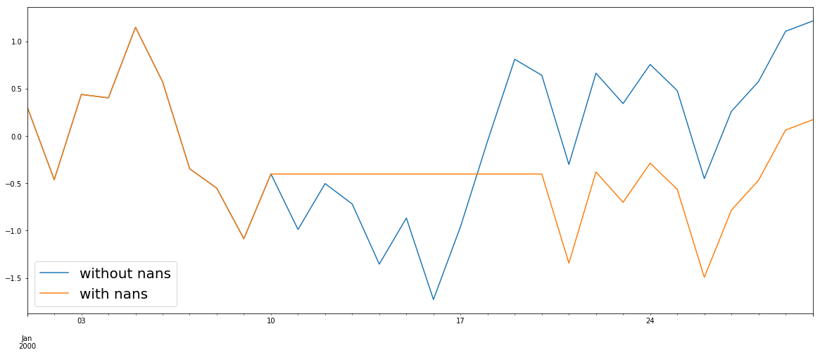

ts.count()

ts.notnull().sum()

ts.cumsum().fillna(method="ffill").plot()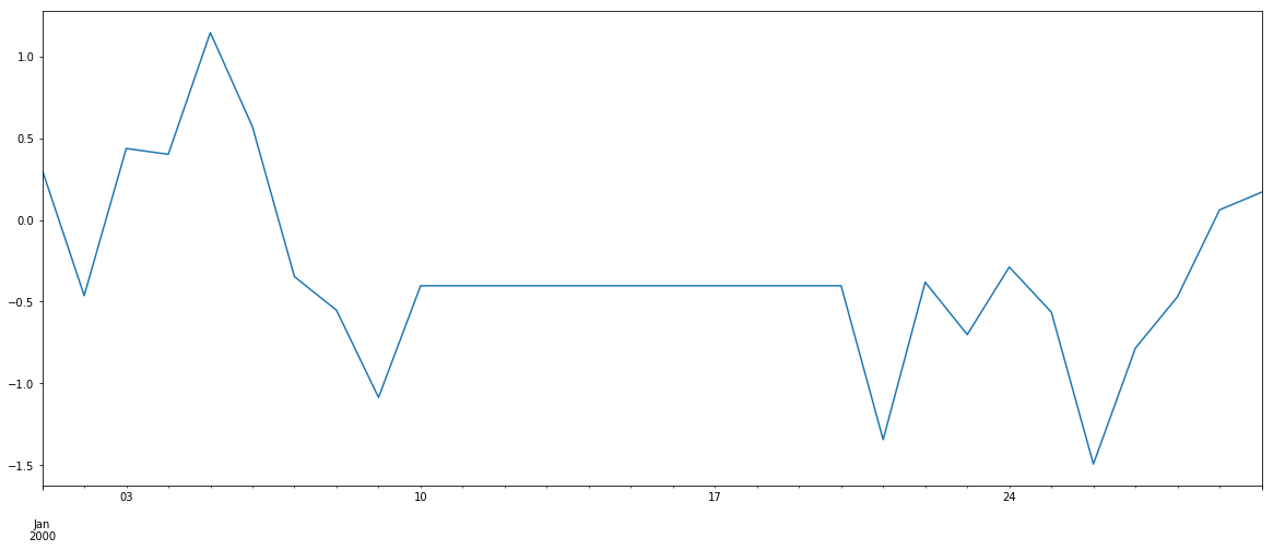

ts.cumsum().fillna(method="ffill", limit=3).plot()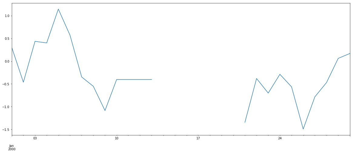

# Anti-causal fill!
ts.cumsum().fillna(method="bfill", limit=3).plot()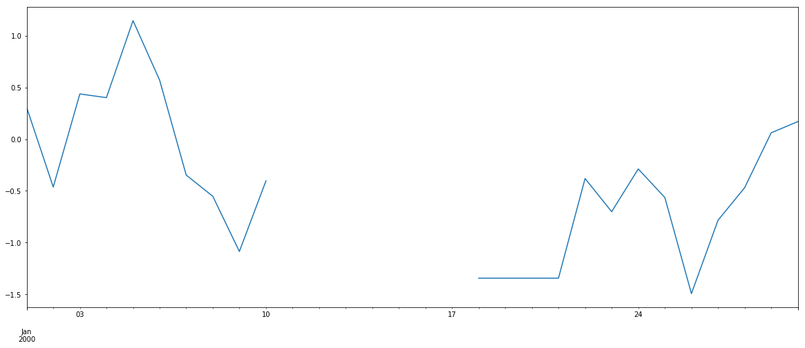

# Before cumsum.
ts.plot()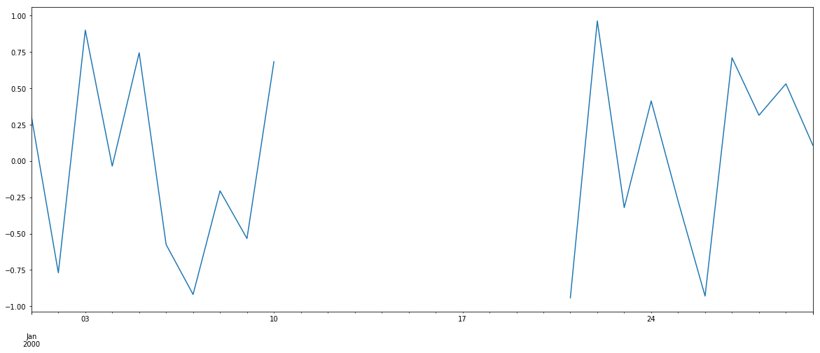

ts.interpolate(method="linear").plot()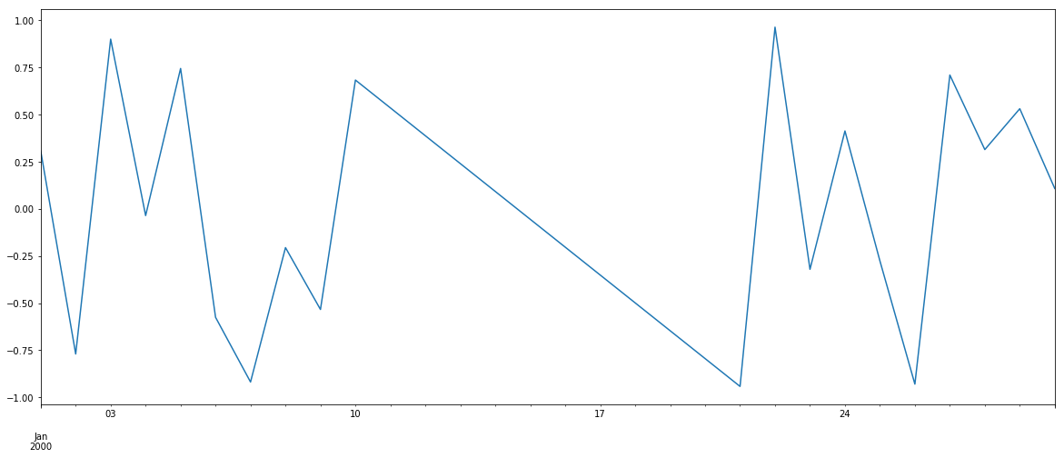

np.random.seed(2)
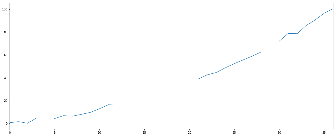
ser = pd.Series(np.arange(1, 10.1, 0.25) ** 2 + np.random.randn(37))
bad = np.array([4, 13, 14, 15, 16, 17, 18, 20, 29])
ser[bad] = np.nan
ser.plot()