Table of Contents
import pandas as pd


def print_ht(df):
    print(df.head())
    print(df.tail())
Time series
Anything that is observed or measured at many points in time
- fixed frequency
- irregular
One can refer to time series in terms of
- timestamps: specific instant in times
- intervals of time: indicated by start / end timestamps
- fixed periods: e.g., months of 2010, years
- This is a special case of “interval of time”
- delta times with respect to a beginning of time
Date and time data types and tools
- date
- time
- datetime
- timedelta
from datetime import datetime, timedelta

now = datetime.now()
print("now=", now)
print(now.year, now.month, now.day)
now= 2018-05-13 10:54:40.633243
2018 5 13
delta = datetime(2011, 1, 7) - datetime(2008, 6, 25, 8, 15)
print("delta=", delta)
print(delta.days, delta.seconds)
delta= 925 days, 15:45:00
925 56700
start = datetime(2011, 1, 7)
print(start + timedelta(12))
2011-01-19 00:00:00
Converting between string and datetime
ts = datetime(2011, 1, 3)

print("str=", str(ts))
# Format using ISO C89.
# strftime = str Format time
print("strftime=", ts.strftime("%Y-%m-%d"))
str= 2011-01-03 00:00:00
strftime= 2011-01-03
# strptime = str Parse time
# It is useful to parse a date in a known format.
value = "2011-01-03"
datetime.strptime(value, "%Y-%m-%d")
datetime.datetime(2011, 1, 3, 0, 0)# To parse data in unknown format.
import dateutil
print(dateutil.parser.parse("2011-01-03"))
print(dateutil.parser.parse("Jan 31, 1997 10:45 PM"))
# Using pandas.
print(pd.to_datetime("2011-07-06 12:00:00"))2011-01-03 00:00:00
1997-01-31 22:45:00
2011-07-06 12:00:00
# pd.to_datetime works also with array of strings.
datestrs = ["2011-07-06 12:00:00", "2011-08-06 00:00:00"]
print(pd.to_datetime(datestrs))
DatetimeIndex(['2011-07-06 12:00:00', '2011-08-06 00:00:00'], dtype='datetime64[ns]', freq=None)
# None gets converted into a Not-A-Time.
print(pd.to_datetime(datestrs + [None]))
DatetimeIndex(['2011-07-06 12:00:00', '2011-08-06 00:00:00', 'NaT'], dtype='datetime64[ns]', freq=None)
Time series basics
dates = [
    datetime(2011, 1, 2),
    datetime(2011, 1, 5),
    datetime(2011, 1, 7),
    datetime(2011, 1, 8),
    datetime(2011, 1, 10),
    datetime(2011, 1, 12),
]

ts = pd.Series(np.random.randn(6), index=dates)

ts
2011-01-02 -0.195830
2011-01-05 -0.813747
2011-01-07 0.967337
2011-01-08 -0.868878
2011-01-10 2.101715
2011-01-12 0.558378
dtype: float64ts.indexDatetimeIndex(['2011-01-02', '2011-01-05', '2011-01-07', '2011-01-08',
'2011-01-10', '2011-01-12'],
dtype='datetime64[ns]', freq=None)# Arithmetic operations between differently indexed time series
# automatically align on dates.
ts + ts[::2]2011-01-02 -0.391659
2011-01-05 NaN
2011-01-07 1.934673
2011-01-08 NaN
2011-01-10 4.203429
2011-01-12 NaN
dtype: float64ts[::2]2011-01-02 -0.195830
2011-01-07 0.967337
2011-01-10 2.101715
dtype: float64# Timestamps are stored using np datetime64 at ns resolution.
print("ts.index.dtype=", ts.index.dtype)
# Timestamp are derived from datetime objects.
timestamp = ts.index[0]
print(type(timestamp))
print(timestamp)ts.index.dtype= datetime64[ns]
<class 'pandas._libs.tslib.Timestamp'>
2011-01-02 00:00:00
Indexing, selection, subsetting
# Time series behaves as any pd.Series.
print("ts=\n", ts)
stamp = ts.index[2]
print("\nstamp=", stamp)ts=
2011-01-02   -0.195830
2011-01-05   -0.813747
2011-01-07    0.967337
2011-01-08   -0.868878
2011-01-10    2.101715
2011-01-12    0.558378
dtype: float64
stamp= 2011-01-07 00:00:00
# You can pass a string that will be interpreted as a date.

print(ts["1/10/2011"])

print(ts["20110110"])
2.10171465932
2.10171465932
longer_ts = pd.Series(
    np.random.randn(1000), index=pd.date_range("1/1/2000", periods=1000)
)

print_ht(longer_ts)
2000-01-01 0.953442
2000-01-02 2.228868
2000-01-03 -1.962444
2000-01-04 -0.484121
2000-01-05 -0.616139
Freq: D, dtype: float64
2002-09-22 0.499749
2002-09-23 -0.365132
2002-09-24 -2.176054
2002-09-25 -0.294013
2002-09-26 -1.913276
Freq: D, dtype: float64
# Filter by year.
print_ht(longer_ts["2001"])
2001-01-01 -0.026238
2001-01-02 0.174582
2001-01-03 -0.522434
2001-01-04 0.246643
2001-01-05 0.622896
Freq: D, dtype: float64
2001-12-27 0.538356
2001-12-28 0.995585
2001-12-29 0.536215
2001-12-30 -0.026049
2001-12-31 -1.058872
Freq: D, dtype: float64
# Filter by month.
print_ht(longer_ts["2001-05"])
2001-05-01 -1.382761
2001-05-02 0.364104
2001-05-03 -0.243860
2001-05-04 1.489501
2001-05-05 0.469970
Freq: D, dtype: float64
2001-05-27 -0.039531
2001-05-28 0.911845
2001-05-29 -1.164597
2001-05-30 -2.296297
2001-05-31 0.173897
Freq: D, dtype: float64
# Slice by datetime.
ts[datetime(2011, 1, 7) :]
2011-01-07 0.967337
2011-01-08 -0.868878
2011-01-10 2.101715
2011-01-12 0.558378
dtype: float64# One can use date, datetime, or timestamp to slice.
# Note that slicing creates a np view on the object, and there
# is no data copied.
ts["1/6/2011":"1/11/2011"]2011-01-07 0.967337
2011-01-08 -0.868878
2011-01-10 2.101715
dtype: float64ts.truncate(after="1/9/2011")2011-01-02 -0.195830
2011-01-05 -0.813747
2011-01-07 0.967337
2011-01-08 -0.868878
dtype: float64# Everything works also for DataFrame indexed on datetimes.
dates = pd.date_range("1/1/2000", periods=100, freq="W-WED")
long_df = pd.DataFrame(
np.random.randn(100, 4),
index=dates,
columns="Colorado Texas NY Ohio".split(),
)
print(long_df.index.is_unique)
print_ht(long_df)True
Colorado Texas NY Ohio
2000-01-05 0.228642 0.203085 -0.322465 -1.242223
2000-01-12 0.882768 -0.119918 0.345217 2.635342
2000-01-19 -1.286971 -1.705926 -0.597030 0.063292
2000-01-26 -1.317127 0.366290 0.492232 1.966448
2000-02-02 -0.784780 0.629830 -0.646747 -0.466076
Colorado Texas NY Ohio
2001-10-31 0.039872 -0.905562 -0.188492 0.116938
2001-11-07 -1.212310 0.267614 1.345367 -0.770098
2001-11-14 0.901416 -1.286568 -0.711707 -1.612438
2001-11-21 -0.546983 -0.653516 0.026749 -1.293937
2001-11-28 0.577820 -0.985672 -1.704768 0.277601
long_df.loc["5-2001"]Loading...
Time series with duplicated indices.
dates = pd.DatetimeIndex(
    ["1/1/2000", "1/2/2000", "1/2/2000", "1/2/2000", "1/3/2000"]
)

dup_ts = pd.Series(np.arange(5), index=dates)

dup_ts
2000-01-01 0
2000-01-02 1
2000-01-02 2
2000-01-02 3
2000-01-03 4
dtype: int64dup_ts.index.is_uniqueFalse# Indexing can produce scalar values or slices, depending on whether
# a timestamp is duplicated.
# Not dup.
print(dup_ts["1/3/2000"])
# Dup.
print(dup_ts["1/2/2000"])4
2000-01-02 1
2000-01-02 2
2000-01-02 3
dtype: int64
# To aggregate the data, you can use groupby using level=0.
grouped = dup_ts.groupby(level=0)

# Count elements per date.
print(grouped.count())

# Compute mean.
print(grouped.mean())
2000-01-01 1
2000-01-02 3
2000-01-03 1
dtype: int64
2000-01-01 0
2000-01-02 2
2000-01-03 4
dtype: int64
Date ranges, freqs, shifting
# Time series in Pandas are assumed to be "irregular", i.e., having
# no fixed frequency.
# Often we want to work with time series with fixed frequency.
# Pandas has functions for:
# - resampling
# - inferring frequencies
# - generating fixed-frequency ranges
dates = [
datetime(2011, 1, 2),
datetime(2011, 1, 5),
datetime(2011, 1, 7),
datetime(2011, 1, 8),
datetime(2011, 1, 10),
datetime(2011, 1, 12),
]
ts = pd.Series(np.random.randn(6), index=dates)
ts2011-01-02 -1.420990
2011-01-05 0.674290
2011-01-07 0.712650
2011-01-08 -0.635353
2011-01-10 0.732992
2011-01-12 0.904861
dtype: float64ts.resample("D")DatetimeIndexResampler [freq=<Day>, axis=0, closed=left, label=left, convention=start, base=0]Generating date ranges
# Sample daily (by default) a (closed) interval of dates.
pd.date_range("2012-04-01", "2012-06-01")
DatetimeIndex(['2012-04-01', '2012-04-02', '2012-04-03', '2012-04-04',
'2012-04-05', '2012-04-06', '2012-04-07', '2012-04-08',
'2012-04-09', '2012-04-10', '2012-04-11', '2012-04-12',
'2012-04-13', '2012-04-14', '2012-04-15', '2012-04-16',
'2012-04-17', '2012-04-18', '2012-04-19', '2012-04-20',
'2012-04-21', '2012-04-22', '2012-04-23', '2012-04-24',
'2012-04-25', '2012-04-26', '2012-04-27', '2012-04-28',
'2012-04-29', '2012-04-30', '2012-05-01', '2012-05-02',
'2012-05-03', '2012-05-04', '2012-05-05', '2012-05-06',
'2012-05-07', '2012-05-08', '2012-05-09', '2012-05-10',
'2012-05-11', '2012-05-12', '2012-05-13', '2012-05-14',
'2012-05-15', '2012-05-16', '2012-05-17', '2012-05-18',
'2012-05-19', '2012-05-20', '2012-05-21', '2012-05-22',
'2012-05-23', '2012-05-24', '2012-05-25', '2012-05-26',
'2012-05-27', '2012-05-28', '2012-05-29', '2012-05-30',
'2012-05-31', '2012-06-01'],
dtype='datetime64[ns]', freq='D')# If only one point of the interval is specified, periods is
# required
print(pd.date_range(start="2012-04-01", periods=5))
print(pd.date_range(end="2012-06-01", periods=5))DatetimeIndex(['2012-04-01', '2012-04-02', '2012-04-03', '2012-04-04',
'2012-04-05'],
dtype='datetime64[ns]', freq='D')
DatetimeIndex(['2012-05-28', '2012-05-29', '2012-05-30', '2012-05-31',
'2012-06-01'],
dtype='datetime64[ns]', freq='D')
pd.date_range("2000-01-01", "2000-06-01", freq="BM")DatetimeIndex(['2000-01-31', '2000-02-29', '2000-03-31', '2000-04-28',
'2000-05-31'],
dtype='datetime64[ns]', freq='BM')# date_range() preserves the time, if present.
pd.date_range("2012-05-02 12:56:31", periods=5)DatetimeIndex(['2012-05-02 12:56:31', '2012-05-03 12:56:31',
'2012-05-04 12:56:31', '2012-05-05 12:56:31',
'2012-05-06 12:56:31'],
dtype='datetime64[ns]', freq='D')# normalize=True aligns on midnights.
pd.date_range("2012-05-02 12:56:31", periods=5, normalize=True)DatetimeIndex(['2012-05-02', '2012-05-03', '2012-05-04', '2012-05-05',
'2012-05-06'],
dtype='datetime64[ns]', freq='D')Frequencies and date offsets
- frequencies are composed of a base frequency and a multiplier
from pandas.tseries.offsets import Hour, Minute

hour = Hour()
print(hour)
<Hour>
four_hours = Hour(4)
print(four_hours)
<4 * Hours>
pd.date_range("2000-01-01", "2000-01-02 23:59", freq="4h")DatetimeIndex(['2000-01-01 00:00:00', '2000-01-01 04:00:00',
'2000-01-01 08:00:00', '2000-01-01 12:00:00',
'2000-01-01 16:00:00', '2000-01-01 20:00:00',
'2000-01-02 00:00:00', '2000-01-02 04:00:00',
'2000-01-02 08:00:00', '2000-01-02 12:00:00',
'2000-01-02 16:00:00', '2000-01-02 20:00:00'],
dtype='datetime64[ns]', freq='4H')# Frequencies can be combined.
Hour(2) + Minute(30)<150 * Minutes>pd.date_range("2000-01-01", periods=10, freq="1h30min")DatetimeIndex(['2000-01-01 00:00:00', '2000-01-01 01:30:00',
'2000-01-01 03:00:00', '2000-01-01 04:30:00',
'2000-01-01 06:00:00', '2000-01-01 07:30:00',
'2000-01-01 09:00:00', '2000-01-01 10:30:00',
'2000-01-01 12:00:00', '2000-01-01 13:30:00'],
dtype='datetime64[ns]', freq='90T')# Week of month: e.g., 3rd Friday of each month.
pd.date_range("2012-01-01", "2012-09-01", freq="WOM-3FRI")DatetimeIndex(['2012-01-20', '2012-02-17', '2012-03-16', '2012-04-20',
'2012-05-18', '2012-06-15', '2012-07-20', '2012-08-17'],
dtype='datetime64[ns]', freq='WOM-3FRI')Shifting data
- shift is about moving data back and forward through time
ts = pd.Series(
    np.random.randn(4), index=pd.date_range("1/1/2000", periods=4, freq="M")
)
ts
2000-01-31 0.137219
2000-02-29 -0.441725
2000-03-31 -0.025440
2000-04-30 -0.647758
Freq: M, dtype: float64# Shift backward 2 lags (delay).
# Note that no new timestamps is inferred, so data is lost.
ts.shift(2)2000-01-31 NaN
2000-02-29 NaN
2000-03-31 0.137219
2000-04-30 -0.441725
Freq: M, dtype: float64# Shift forward 2 lags.
ts.shift(-2)2000-01-31 -0.025440
2000-02-29 -0.647758
2000-03-31 NaN
2000-04-30 NaN
Freq: M, dtype: float64# If frequency of data is known, new timestamps can be inferred.
ts.shift(2, freq="M")2000-03-31 0.137219
2000-04-30 -0.441725
2000-05-31 -0.025440
2000-06-30 -0.647758
Freq: M, dtype: float64ts.shift(3, freq="D")2000-02-03 0.137219
2000-03-03 -0.441725
2000-04-03 -0.025440
2000-05-03 -0.647758
dtype: float64# Shift back of 4 * 90 mins = 6hrs.
ts.shift(4, freq="90T")2000-01-31 06:00:00 0.137219
2000-02-29 06:00:00 -0.441725
2000-03-31 06:00:00 -0.025440
2000-04-30 06:00:00 -0.647758
Freq: M, dtype: float64Shifting dates with offsets
from pandas.tseries.offsets import Day, MonthEnd

now = datetime(2011, 11, 17)

print(now + 3 * Day())
2011-11-20 00:00:00
# Anchored offsets allow to align a period of time.
print(now + MonthEnd())
# This is equivalent to:
print(MonthEnd().rollforward(now))
2011-11-30 00:00:00
2011-11-30 00:00:00
print(now + MonthEnd(2))2011-12-31 00:00:00
# One can use date offsets with groupby.
ts = pd.Series(
    np.random.randn(20), index=pd.date_range("1/15/2000", periods=20, freq="4d")
)
ts
2000-01-15 0.081999
2000-01-19 0.864714
2000-01-23 0.284556
2000-01-27 0.433515
2000-01-31 1.967312
2000-02-04 -0.461309
2000-02-08 -0.939936
2000-02-12 -0.393808
2000-02-16 -0.057009
2000-02-20 -0.408874
2000-02-24 1.047092
2000-02-28 -1.146174
2000-03-03 2.388882
2000-03-07 0.578028
2000-03-11 -0.825274
2000-03-15 -0.332605
2000-03-19 -2.258880
2000-03-23 1.960624
2000-03-27 -0.228699
2000-03-31 -0.369610
Freq: 4D, dtype: float64offset = MonthEnd()
def print_group(df):
print("[%s, %s]" % (df.index[0], df.index[-1]))
# print ts.groupby(offset.rollforward).first()
# print ts.groupby(offset.rollforward).last()
_ = ts.groupby(offset.rollforward).agg(print_group)[2000-01-15 00:00:00, 2000-01-31 00:00:00]
[2000-02-04 00:00:00, 2000-02-28 00:00:00]
[2000-03-03 00:00:00, 2000-03-31 00:00:00]
# This is equivalent to resample.
ts.resample("M").agg(print_group)
[2000-01-15 00:00:00, 2000-01-31 00:00:00]
[2000-02-04 00:00:00, 2000-02-28 00:00:00]
[2000-03-03 00:00:00, 2000-03-31 00:00:00]
Time zone handling
- Working with time zones is unpleasant
- One can work with UTC (Coordinated Universal Time), which is an international standard
- Time zones are expressed as offsets from UTC
- E.g., NY is +4 during daylight saving time (DST), +5 otherwise
- pytz is 3rd party library
- Olson db
- DST and UTC offsets have been changed many times
- pandas wraps pytz
import pytz

pytz.common_timezones[-7:]
['US/Arizona',
'US/Central',
'US/Eastern',
'US/Hawaii',
'US/Mountain',
'US/Pacific',
'UTC']tz = pytz.timezone("America/New_York")
print(tz)
print(repr(tz))America/New_York
<DstTzInfo 'America/New_York' LMT-1 day, 19:04:00 STD>
Time zone localization and conversion
- By default time series are time zone naive
rng = pd.date_range("3/9/2012 9:30", periods=6, freq="D")

print(rng)

# Note that tz field is none.
print(rng.tz)
DatetimeIndex(['2012-03-09 09:30:00', '2012-03-10 09:30:00',
'2012-03-11 09:30:00', '2012-03-12 09:30:00',
'2012-03-13 09:30:00', '2012-03-14 09:30:00'],
dtype='datetime64[ns]', freq='D')
None
ts = pd.Series(np.random.randn(len(rng)), index=rng)
print(ts)

# Note that tz field is none.
print("index.tz=", ts.index.tz)
2012-03-09 09:30:00 0.659952
2012-03-10 09:30:00 -0.277512
2012-03-11 09:30:00 -0.584728
2012-03-12 09:30:00 -0.039433
2012-03-13 09:30:00 0.790273
2012-03-14 09:30:00 -0.326480
Freq: D, dtype: float64
index.tz= None
# Generate data range with a UTC time zone.
rng = pd.date_range("3/9/2012 9:30", periods=6, freq="D", tz="UTC")

print(rng)
print(rng.tz)
DatetimeIndex(['2012-03-09 09:30:00+00:00', '2012-03-10 09:30:00+00:00',
'2012-03-11 09:30:00+00:00', '2012-03-12 09:30:00+00:00',
'2012-03-13 09:30:00+00:00', '2012-03-14 09:30:00+00:00'],
dtype='datetime64[ns, UTC]', freq='D')
UTC
# Generate data range with a time zone.
rng = pd.date_range("3/9/2012 9:30", periods=6, freq="D", tz="US/Pacific")

print(rng)
print(rng.tz)
DatetimeIndex(['2012-03-09 09:30:00-08:00', '2012-03-10 09:30:00-08:00',
'2012-03-11 09:30:00-07:00', '2012-03-12 09:30:00-07:00',
'2012-03-13 09:30:00-07:00', '2012-03-14 09:30:00-07:00'],
dtype='datetime64[ns, US/Pacific]', freq='D')
US/Pacific
# Naive times can be converted in "localized".
ts_utc = ts.tz_localize("UTC")
print(ts_utc)
print(ts_utc.index.tz)

# Once they are localized, dates can be converted into other time zones.
ts_edt = ts_utc.tz_convert("America/New_York")
print("\n", ts_edt)
print(ts_edt.index.tz)
2012-03-09 09:30:00+00:00 0.659952
2012-03-10 09:30:00+00:00 -0.277512
2012-03-11 09:30:00+00:00 -0.584728
2012-03-12 09:30:00+00:00 -0.039433
2012-03-13 09:30:00+00:00 0.790273
2012-03-14 09:30:00+00:00 -0.326480
Freq: D, dtype: float64
UTC
2012-03-09 04:30:00-05:00 0.659952
2012-03-10 04:30:00-05:00 -0.277512
2012-03-11 05:30:00-04:00 -0.584728
2012-03-12 05:30:00-04:00 -0.039433
2012-03-13 05:30:00-04:00 0.790273
2012-03-14 05:30:00-04:00 -0.326480
Freq: D, dtype: float64
America/New_York
# Add a ET timezone.
ts_edt = ts.tz_localize("America/New_York")
print(ts_edt)
print(ts_edt.index.tz)
2012-03-09 09:30:00-05:00 0.659952
2012-03-10 09:30:00-05:00 -0.277512
2012-03-11 09:30:00-04:00 -0.584728
2012-03-12 09:30:00-04:00 -0.039433
2012-03-13 09:30:00-04:00 0.790273
2012-03-14 09:30:00-04:00 -0.326480
Freq: D, dtype: float64
America/New_York
# tz_localize and tz_convert are also methods of DateTimeIndexOperations with time zone-aware timestamp objects
- Also Timestamp can be handled in terms of time-zones
ts = pd.Timestamp("2011-03-12 04:00")
print("ts=", ts)

ts_utc = ts.tz_localize("UTC")
print("\nts_utc=", ts_utc)

print("ts_convert=", ts_utc.tz_convert("America/New_York"))
ts= 2011-03-12 04:00:00
ts_utc= 2011-03-12 04:00:00+00:00
ts_convert= 2011-03-11 23:00:00-05:00
ts_moscow = pd.Timestamp("2011-03-12 04:00", tz="Europe/Moscow")
print(ts_moscow)
2011-03-12 04:00:00+03:00
# Tz-aware Timestamp objects are stored a nanoseconds since Unix epoch (1970-01-01).
# This is not changed when tz conversions are applied.

print(ts_utc)
print(type(ts_utc))
print(ts_utc.value)
print(ts_utc.tz_convert("America/New_York").value)
2011-03-12 04:00:00+00:00
<class 'pandas._libs.tslib.Timestamp'>
1299902400000000000
1299902400000000000
Operations between different time zones
- If two time series with different time zones are combined, the result is UTC
rng = pd.date_range("3/7/2012 9:30", periods=6, freq="B")
ts = pd.Series(np.random.randn(len(rng)), index=rng)
print(ts)
2012-03-07 09:30:00 0.023061
2012-03-08 09:30:00 0.285329
2012-03-09 09:30:00 -1.310567
2012-03-12 09:30:00 2.882604
2012-03-13 09:30:00 0.921431
2012-03-14 09:30:00 0.277645
Freq: B, dtype: float64
ts1 = ts.tz_localize("Europe/London")
ts2 = ts1.tz_convert("Europe/Moscow")

print(ts1)
print(ts2)
2012-03-07 09:30:00+00:00 0.023061
2012-03-08 09:30:00+00:00 0.285329
2012-03-09 09:30:00+00:00 -1.310567
2012-03-12 09:30:00+00:00 2.882604
2012-03-13 09:30:00+00:00 0.921431
2012-03-14 09:30:00+00:00 0.277645
Freq: B, dtype: float64
2012-03-07 13:30:00+04:00 0.023061
2012-03-08 13:30:00+04:00 0.285329
2012-03-09 13:30:00+04:00 -1.310567
2012-03-12 13:30:00+04:00 2.882604
2012-03-13 13:30:00+04:00 0.921431
2012-03-14 13:30:00+04:00 0.277645
Freq: B, dtype: float64
print(ts1 + ts2)2012-03-07 09:30:00+00:00 0.046122
2012-03-08 09:30:00+00:00 0.570658
2012-03-09 09:30:00+00:00 -2.621134
2012-03-12 09:30:00+00:00 5.765209
2012-03-13 09:30:00+00:00 1.842862
2012-03-14 09:30:00+00:00 0.555290
Freq: B, dtype: float64
Periods and period arithmetic
- Periods represent timespans (e.g., days, months, quarters, years)
# Freq is the same frequencies used for other applications.

# E.g., 'A-DEC' means annual dates anchored to the end last cander of Dec.
p = pd.Period(2007, freq="A-DEC")
p
Period('2007', 'A-DEC')p + 5Period('2012', 'A-DEC')p - 2Period('2005', 'A-DEC')# Distance of periods in terms of periods.
p2 = pd.Period("2014", freq="A-DEC")
print("p2=", p2)
print("p =", p)
print("p2-p=", p2 - p)p2= 2014
p = 2007
p2-p= 7
# Date range with monthly cadence.
rng1 = pd.date_range("2000-01-01", "2000-06-30", freq="M")
print(rng1)
DatetimeIndex(['2000-01-31', '2000-02-29', '2000-03-31', '2000-04-30',
'2000-05-31', '2000-06-30'],
dtype='datetime64[ns]', freq='M')
ts1 = pd.Series(np.random.randn(len(rng1)), index=rng1)
print(ts1)

print(type(ts1.index))
print(type(ts1.index[0]))
2000-01-31 -0.241163
2000-02-29 -0.304942
2000-03-31 -0.107074
2000-04-30 -0.572908
2000-05-31 -0.165864
2000-06-30 1.062376
Freq: M, dtype: float64
<class 'pandas.core.indexes.datetimes.DatetimeIndex'>
<class 'pandas._libs.tslib.Timestamp'>
# Period range with monthly cadence.
rng2 = pd.period_range("2000-01-01", "2000-06-30", freq="M")
print(rng2)
PeriodIndex(['2000-01', '2000-02', '2000-03', '2000-04', '2000-05', '2000-06'], dtype='period[M]', freq='M')
# A PeriodIndex stores a sequence of periods
# It can be used as an axis index, like a DatetimeIndex.
ts2 = pd.Series(np.random.randn(len(rng2)), index=rng2)
print(ts2)

print(type(ts2.index))
print(type(ts2.index[0]))
2000-01 0.993906
2000-02 -0.645846
2000-03 1.465864
2000-04 0.334810
2000-05 -0.035259
2000-06 0.064194
Freq: M, dtype: float64
<class 'pandas.core.indexes.period.PeriodIndex'>
<class 'pandas._libs.period.Period'>
values = ["2001Q3", "2002Q2", "2003Q1"]

index = pd.PeriodIndex(values, freq="Q-DEC")
print(index)
PeriodIndex(['2001Q3', '2002Q2', '2003Q1'], dtype='period[Q-DEC]', freq='Q-DEC')
Period frequency conversion
- One can convert a PeriodIndex to another frequency
# A period for 2007 anchored to end of Dec.
p = pd.Period("2007", freq="A-DEC")
p
Period('2007', 'A-DEC')p.asfreq("M", how="start")Period('2007-01', 'M')p.asfreq("M", how="end")Period('2007-12', 'M')# Consider a year ending at the end of June.
p = pd.Period("2007", "A-JUN")
pPeriod('2007', 'A-JUN')p.asfreq("M", how="start")Period('2006-07', 'M')p.asfreq("M", how="end")Period('2007-06', 'M')# Also PeriodIndex can be converted to
rng = pd.period_range("2006", "2009", freq="A-DEC")
ts = pd.Series(np.random.randn(len(rng)), index=rng)
print(ts)2006 -1.079111
2007 -1.036980
2008 0.597151
2009 1.686564
Freq: A-DEC, dtype: float64
# Pick the first month of the year period ending in Dec.
ts.asfreq("M", how="start")
2006-01 -1.079111
2007-01 -1.036980
2008-01 0.597151
2009-01 1.686564
Freq: M, dtype: float64# Use the last business day of the period.
ts.asfreq("B", how="end")2006-12-29 -1.079111
2007-12-31 -1.036980
2008-12-31 0.597151
2009-12-31 1.686564
Freq: B, dtype: float64Quarterly period frequencies
- Quarterly data is standard in accounting and finance
- Quarterly data is reported relative to fiscal year end (typically the last calendar or business day of one of the 12 months of the year)
# 4th quarter, with fiscal year end in Jan.
p = pd.Period("2012Q4", freq="Q-JAN")
p
Period('2012Q4', 'Q-JAN')# The 4th quarter is:
p.asfreq("D", "start"), p.asfreq("D", "end")(Period('2011-11-01', 'D'), Period('2012-01-31', 'D'))# Get a timestamp at 4pm on second-to-last business day of the quarter.
ts = (p.asfreq("B", "end") - 1).asfreq("T", "s") + 16 * 60
print(ts)2012-01-30 16:00
Converting timestamps to periods (and back)
- periods always refer to non-overlapping timestamps
- a timestamp can only belong to a single period for a given frequency
rng = pd.date_range("1/1/2000", periods=3, freq="M")
rng
DatetimeIndex(['2000-01-31', '2000-02-29', '2000-03-31'], dtype='datetime64[ns]', freq='M')ts = pd.Series(randn(3), index=rng)
ts2000-01-31 -0.456340
2000-02-29 -0.400942
2000-03-31 0.585983
Freq: M, dtype: float64# to_period() infers the frequency automatically
# In practice it uses the same frequency of the timeseries.
pts = ts.to_period()
print(pts)2000-01 -0.456340
2000-02 -0.400942
2000-03 0.585983
Freq: M, dtype: float64
rng = pd.date_range("1/29/2000", periods=6, freq="D")
ts2 = pd.Series(randn(6), index=rng)

print(ts2)
2000-01-29 -0.785957
2000-01-30 1.272619
2000-01-31 0.180610
2000-02-01 0.700050
2000-02-02 -0.423228
2000-02-03 0.260495
Freq: D, dtype: float64
# Convert each timestamp to the including period.
# Note that the frequency of timestamp and periods are different.
ts2.to_period("M")
2000-01 -0.785957
2000-01 1.272619
2000-01 0.180610
2000-02 0.700050
2000-02 -0.423228
2000-02 0.260495
Freq: M, dtype: float64pts2 = ts2.to_period()
print(pts2)2000-01-29 -0.785957
2000-01-30 1.272619
2000-01-31 0.180610
2000-02-01 0.700050
2000-02-02 -0.423228
2000-02-03 0.260495
Freq: D, dtype: float64
pts2.indexPeriodIndex(['2000-01-29', '2000-01-30', '2000-01-31', '2000-02-01',
'2000-02-02', '2000-02-03'],
dtype='period[D]', freq='D')# Converting back to timestamps.
pts2 = ts2.to_period("M")
print(pts2)
print(pts2.to_timestamp(how="end"))2000-01 -0.785957
2000-01 1.272619
2000-01 0.180610
2000-02 0.700050
2000-02 -0.423228
2000-02 0.260495
Freq: M, dtype: float64
2000-01-31 -0.785957
2000-01-31 1.272619
2000-01-31 0.180610
2000-02-29 0.700050
2000-02-29 -0.423228
2000-02-29 0.260495
dtype: float64
Creating a PeriodIndex from arrays
- If the timespan information are stored in multiple columns, the constructor of PeriodIndex can gather them and use them
!ls /Users/gp/src/github/pydata-book/examplesarray_ex.txt macrodata.csv
csv_mindex.csv out.csv
ex1.csv segismundo.txt
ex1.xlsx spx.csv
ex2.csv stinkbug.png
ex3.csv stock_px.csv
ex3.txt stock_px_2.csv
ex4.csv test_file.csv
ex5.csv tips.csv
ex6.csv tseries.csv
ex7.csv volume.csv
example.json yahoo_price.pkl
fdic_failed_bank_list.html yahoo_volume.pkl
ipython_bug.py
data = pd.read_csv("~/src/github/pydata-book/examples/macrodata.csv")
data.head()
Loading...
print(data.head()[["year", "quarter"]]) year quarter
0 1959.0 1.0
1 1959.0 2.0
2 1959.0 3.0
3 1959.0 4.0
4 1960.0 1.0
index = pd.PeriodIndex(year=data.year, quarter=data.quarter, freq="Q-DEC")

print(index)
PeriodIndex(['1959Q1', '1959Q2', '1959Q3', '1959Q4', '1960Q1', '1960Q2',
'1960Q3', '1960Q4', '1961Q1', '1961Q2',
...
'2007Q2', '2007Q3', '2007Q4', '2008Q1', '2008Q2', '2008Q3',
'2008Q4', '2009Q1', '2009Q2', '2009Q3'],
dtype='period[Q-DEC]', length=203, freq='Q-DEC')
data.index = index
data.infl.head()
1959Q1 0.00
1959Q2 2.34
1959Q3 2.74
1959Q4 0.27
1960Q1 2.31
Freq: Q-DEC, Name: infl, dtype: float64Resampling and frequency conversion
- Resampling = converting a time series from one frequency to another
- Downsampling = aggregating higher frequency data to lower frequency
- Upsampling = converting lower frequency data to higher frequency
- Some operations are not down or upsampling
- E.g., converting from W-WED (weekly on Wednesday) to W-FRI
rng = pd.date_range("1/1/2000", periods=100, freq="D")

ts = pd.Series(randn(len(rng)), index=rng)
ts.head()
2000-01-01 0.290105
2000-01-02 -0.219713
2000-01-03 0.995451
2000-01-04 1.093139
2000-01-05 1.152817
Freq: D, dtype: float64# Resample daily data to monthly using mean to aggregate.
# ts.resample('M', how="mean")
ts.resample("M").mean()2000-01-31 -0.122909
2000-02-29 -0.286706
2000-03-31 0.178215
2000-04-30 0.096529
Freq: M, dtype: float64ts.resample("M", kind="period").mean()2000-01 -0.122909
2000-02 -0.286706
2000-03 0.178215
2000-04 0.096529
Freq: M, dtype: float64- options for resample()
- freq: string (e.g., ‘M’, ‘5min’) or DateOffset (e.g., Second(15)) indicating resampled frequency
- how: function name or function aggregating values
- e.g., mean, ohlc, np.max, first, last, median
- fill_method: how to interpolate when upsampling
- e.g., ffill, bfill
- limit: when filling the maximum number of periods to fill
- closed: in downsampling which end of the interval is closed, i.e., inclusive
- e.g., right, left
- label: in downsampling how to label the aggregated result with the right or left bin edge
- e.g., we can sample 5-min interval [9:30, 9:35) and label it 9:30 or 9:35
- loffset: time adjustment to bin labels to shift aggregate labels
Downsampling
Aggregating data to a regular, lower frequency is a normal time series task
The data doesn’t need to be fixed
- The desired frequency defines bin edges used to aggregate
- Partition
- Each interval is half-open, since each point can only belong to one interval
- The union of all intervals must make up the whole time frame
When sampling
- which side of each interval is closed
- how to label each aggregated bin (beginning or end)
# Generate minute data.
rng = pd.date_range("1/1/2000", periods=12, freq="T")
ts = pd.Series(np.arange(len(rng)), index=rng)

ts
2000-01-01 00:00:00 0
2000-01-01 00:01:00 1
2000-01-01 00:02:00 2
2000-01-01 00:03:00 3
2000-01-01 00:04:00 4
2000-01-01 00:05:00 5
2000-01-01 00:06:00 6
2000-01-01 00:07:00 7
2000-01-01 00:08:00 8
2000-01-01 00:09:00 9
2000-01-01 00:10:00 10
2000-01-01 00:11:00 11
Freq: T, dtype: int64# Aggregate data into 5-min chunks or bars by taking the sum.
# ts.resample('5min', how="sum")
print(ts.resample("5min", closed="left", label="left").sum())
# This is the default.
print(ts.resample("5min").sum())2000-01-01 00:00:00 10
2000-01-01 00:05:00 35
2000-01-01 00:10:00 21
Freq: 5T, dtype: int64
2000-01-01 00:00:00 10
2000-01-01 00:05:00 35
2000-01-01 00:10:00 21
Freq: 5T, dtype: int64
ts.resample("5min", closed="left", label="right").sum()2000-01-01 00:05:00 10
2000-01-01 00:10:00 35
2000-01-01 00:15:00 21
Freq: 5T, dtype: int64ts.resample("5min", closed="right", label="left").sum()1999-12-31 23:55:00 0
2000-01-01 00:00:00 15
2000-01-01 00:05:00 40
2000-01-01 00:10:00 11
Freq: 5T, dtype: int64print(ts.resample("5min", closed="right", label="right").sum())2000-01-01 00:00:00 0
2000-01-01 00:05:00 15
2000-01-01 00:10:00 40
2000-01-01 00:15:00 11
Freq: 5T, dtype: int64
# If you want to shift the index.
# This is equivalent to calling shift() after resampling
ts.resample("5min", how="sum", loffset="-1s")
/Users/gp/.conda/envs/jupyter/lib/python2.7/site-packages/ipykernel_launcher.py:3: FutureWarning: how in .resample() is deprecated
the new syntax is .resample(...).sum()
This is separate from the ipykernel package so we can avoid doing imports until
1999-12-31 23:59:59    10
2000-01-01 00:04:59    35
2000-01-01 00:09:59    21
Freq: 5T, dtype: int64
OHLC resampling
ts.resample("5min").ohlc()Loading...
Resampling with GroupBy
- One can group by and then compute mean
rng = pd.date_range("1/1/2000", periods=100, freq="D")
ts = pd.Series(np.arange(100), index=rng)
print(ts.head())
2000-01-01 0
2000-01-02 1
2000-01-03 2
2000-01-04 3
2000-01-05 4
Freq: D, dtype: int64
ts.groupby(lambda x: x.month).mean()1 15
2 45
3 75
4 95
dtype: int64Upsampling
- When converting from lower to higher frequency, no aggregation is needed
frame = pd.DataFrame(
    np.random.randn(2, 4),
    index=pd.date_range("1/1/2000", periods=2, freq="W-WED"),
    columns="Colorado Texas NY Ohio".split(),
)
frame[:5]
Loading...
# When resampling to daily frequency, missing values are introduced.

# frame.resample("D", fill_method="ffill")
frame.resample("D").ffill()
Loading...
frame.resample("D").ffill(limit=2)Loading...
Resampling with periods
frame = pd.DataFrame(
    np.random.randn(24, 4),
    index=pd.period_range("1-2000", "12-2001", freq="M"),
    columns="Colorado Texas NY Ohio".split(),
)
frame[:5]
Loading...
annual_frame = frame.resample("A-DEC").mean()
annual_frame
Loading...
Time series plotting
!ls ~/src/github/pydata-book/examplesarray_ex.txt macrodata.csv
csv_mindex.csv out.csv
ex1.csv segismundo.txt
ex1.xlsx spx.csv
ex2.csv stinkbug.png
ex3.csv stock_px.csv
ex3.txt stock_px_2.csv
ex4.csv test_file.csv
ex5.csv tips.csv
ex6.csv tseries.csv
ex7.csv volume.csv
example.json yahoo_price.pkl
fdic_failed_bank_list.html yahoo_volume.pkl
ipython_bug.py
close_px_all = pd.read_csv(
    "~/src/github/pydata-book/examples/stock_px.csv",
    index_col=0,
    parse_dates=True,
)

close_px_all.head()
Loading...
close_px = close_px_all["AAPL MSFT XOM".split()]

close_px.head()
Loading...
close_px = close_px.resample("B", fill_method="ffill")/Users/gp/.conda/envs/jupyter/lib/python2.7/site-packages/ipykernel_launcher.py:1: FutureWarning: fill_method is deprecated to .resample()
the new syntax is .resample(...).ffill()
"""Entry point for launching an IPython kernel.
close_px.head()Loading...
close_px["AAPL"].plot()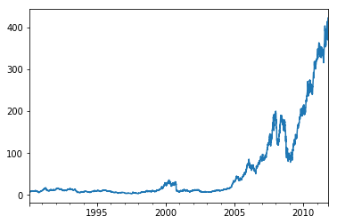
close_px["2009"].plot()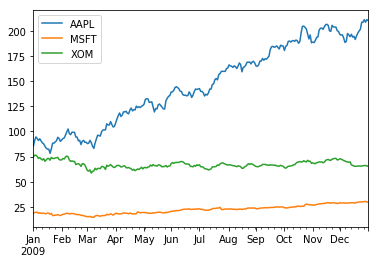
close_px["AAPL"].loc["01-2011":"03-2011"].plot()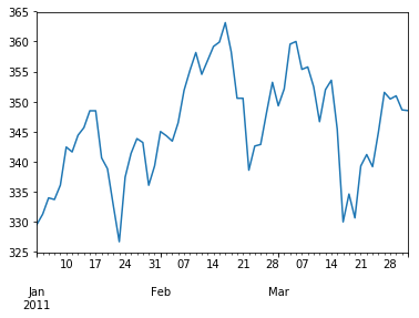
# Quarterly data is nicely formatted with quarterly markers.
# aapl_q = close_px["AAPL"].resample("Q-DEC", fill_method="ffill")
aapl_q = close_px["AAPL"].resample("Q-DEC").ffill()
aapl_q["2009":].plot()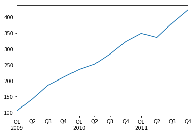
Moving window functions
- Common operations are statistics evaluated over a sliding window, with exponentially decaying weights
close_px.AAPL.plot()

# One needs to specify the number of non-na observations.
# pd.rolling_mean(close_px.AAPL, 250).plot()
close_px.rolling(window=250, center=False).mean().plot()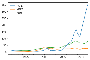
# pd.rolling_std(close_px.AAPL, 250, min_periods=10).plot()
close_px.AAPL.rolling(min_periods=10, window=250, center=False).std().plot()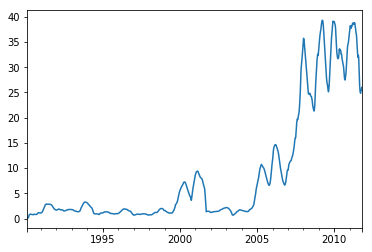
expanding_mean = lambda x: pd.rolling_mean(x, len(x), min_periods=1)# pd.rolling_mean(close_px, 60).plot(logy=True)
close_px.rolling(window=60, center=False).mean().plot(logy=True)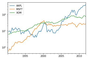
close_px.AAPL.rolling(window=60, center=False).count().plot()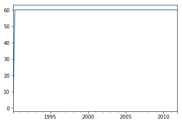
close_px.AAPL.rolling(window=60, center=False).skew().plot()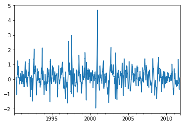
close_px.AAPL.rolling(window=60, center=False).kurt().plot()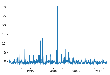
# rolling.apply(): apply a generic function over a moving window
# ewma, ewmvar, ewmstd, ewmcorr, ewmcov: exp-weighted moving *
Exponentially-weighted functions
Instead of specifying a static window size with equally-weighted observations, specify a constant decay factor to give more weight to more reent observations
fig, axes = plt.subplots(
    nrows=1, ncols=1, sharex=True, sharey=True, figsize=(12, 5)
)

aapl_px = close_px.AAPL["2005":"2009"]
ma60 = aapl_px.rolling(60, min_periods=50).mean()
ewma60 = aapl_px.ewm(span=60, min_periods=60).mean()

aapl_px.plot(style="k-", ax=axes)
ma60.plot(style="b--", ax=axes, label="ma")
ewma60.plot(style="r--", ax=axes, label="ewma")

plt.legend()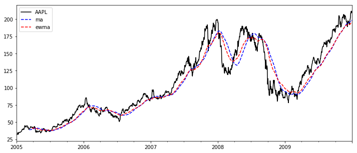
Binary moving window functions
# Some operators (e.g., corr, cov) operate on 2 time series.
spx_px = close_px_all.SPX["2005":"2009"]
spx_rets = spx_px / spx_px.shift(1) - 1

returns = close_px.pct_change()

display(spx_rets.head())
display(returns.head())

# corr = pd.rolling_corr(returns.AAPL, spx_rets, 125, min_periods=100)
corr = returns.AAPL.rolling(125, min_periods=100).corr(spx_rets)
corr.dropna().plot(figsize=(15, 6))
2005-01-03 NaN
2005-01-04 -0.011671
2005-01-05 -0.003628
2005-01-06 0.003506
2005-01-07 -0.001431
Name: SPX, dtype: float64Loading...
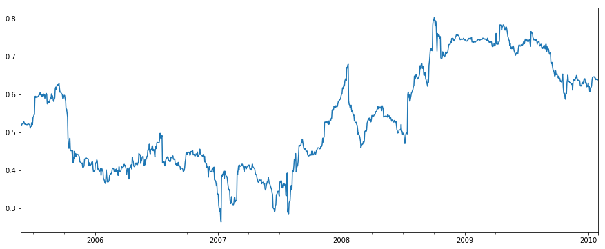
# Multiple columns of a data-frame vs a series.
display(returns.head())
display(spx_rets.head())
corr = returns.rolling(125, min_periods=100).corr(spx_rets)
corr.dropna().plot(figsize=(15, 6))Loading...
2005-01-03         NaN
2005-01-04   -0.011671
2005-01-05   -0.003628
2005-01-06    0.003506
2005-01-07   -0.001431
Name: SPX, dtype: float64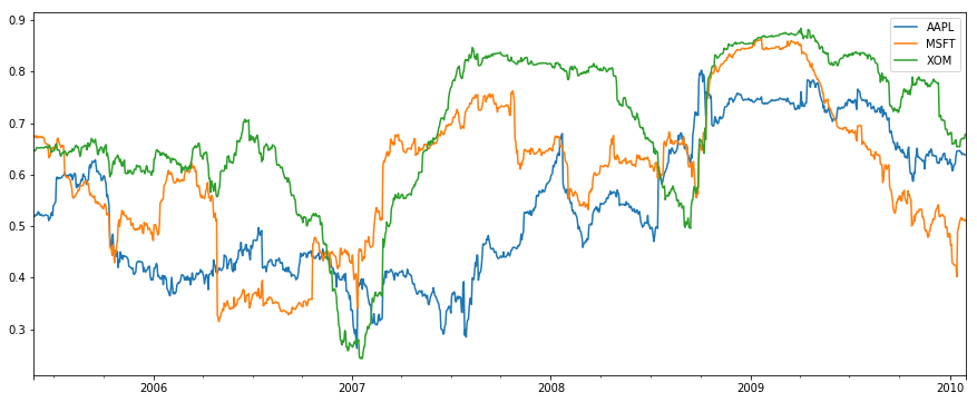
User-defined moving window functions
# rolling_apply)() allows to apply an array function over a moving function.
# The function needs to produce a single function

from scipy.stats import percentileofscore

score_at_2pct = lambda x: percentileofscore(x, 0.02)
# result = pd.rolling_apply(returns.AAPL, 250, score_at_2pct)
# pandas 0.22
result = returns.AAPL.rolling(250).apply(score_at_2pct)

result.plot()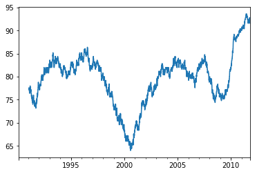
TODO---------------------------------------------------------------------------
NameError Traceback (most recent call last)
<ipython-input-318-9b7105f44b18> in <module>()
----> 1 TODO
NameError: name 'TODO' is not defined