Table of Contents
Imports
!conda info --envs# conda environments:
#
deeplearning /Users/gp/.conda/envs/deeplearning
jupyter * /Users/gp/.conda/envs/jupyter
particleone_teza /Users/gp/.conda/envs/particleone_teza
statarbdeps /Users/gp/.conda/envs/statarbdeps
statarbdeps.20170712-14_11_50 /Users/gp/.conda/envs/statarbdeps.20170712-14_11_50
statarbdeps.20170713-14_06_23 /Users/gp/.conda/envs/statarbdeps.20170713-14_06_23
statarbdeps_base /Users/gp/.conda/envs/statarbdeps_base
statarbdeps_base.20171204-13_21_50 /Users/gp/.conda/envs/statarbdeps_base.20171204-13_21_50
statarbdeps_gp /Users/gp/.conda/envs/statarbdeps_gp
tzdataetlgreen /Users/gp/.conda/envs/tzdataetlgreen
root /opt/teza-conda
import datetime

import numpy as np
import matplotlib.pyplot as plt
import pandas as pd

%matplotlib inline
import notebook_utils
notebook_utils.notebook_config()
# matplotlib.rcParams["figure.figsize"] = (15, 6)
# assert np.__version__ == "1.13.3"
assert pd.__version__ == "0.20.3"
# assert matplotlib.__version__ == "2.0.2"numpy= 1.13.3
pandas= 0.20.3
matplotlib= 2.0.2
sklearn= 0.18.1
# def display_df(df):
# display(df)TODOs
Intro to data structures
Series
- Series is a one-dimensional labeled array holding any data type (integers, strings, floats, objects)
- Axis labels are referred to as the index
np.random.seed(1000)
# Realizations from standard normal.
s = pd.Series(np.random.randn(5))
s
0 -0.804458
1 0.320932
2 -0.025483
3 0.644324
4 -0.300797
dtype: float64np.random.seed(1000)
s = pd.Series(np.random.randn(5), index="a b c d e".split())
sa -0.804458
b 0.320932
c -0.025483
d 0.644324
e -0.300797
dtype: float64# From dictionary.
d = {"a": 0.0, "b": 1.0, "c": 2.0}
s = pd.Series(d)
sa 0.0
b 1.0
c 2.0
dtype: float64DataFrame
df = pd.DataFrame("a b c d e".split())
print("df.index.is_unique=", df.index.is_unique)
print("df.index.is_monotonic=", df.index.is_monotonic)
print("df.index.is_monotonic_increasing=", df.index.is_monotonic_increasing)
df.index.is_unique= True
df.index.is_monotonic= True
df.index.is_monotonic_increasing= True
df = pd.DataFrame("a b c d e".split(), index=[0, 2, 1, 3, 4])
print("df.index.is_unique=", df.index.is_unique)
print("df.index.is_monotonic=", df.index.is_monotonic)
print("df.index.is_monotonic_increasing=", df.index.is_monotonic_increasing)
df.index.is_unique= True
df.index.is_monotonic= False
df.index.is_monotonic_increasing= False
Df from dict
df1 = pd.DataFrame("a b c d".split(), index=[0, 1, 2, 3], columns=["val1"])
dict_ = df1.to_dict()["val1"]
print(dict_)
{0: 'a', 1: 'b', 2: 'c', 3: 'd'}
pd.DataFrame.from_dict({"weight": dict_})Panel
- A panel automatically aligns on union of all indices
Panel from dfs with different indices.
df1 = pd.DataFrame("a b c d".split(), index=[0, 1, 2, 3], columns=["val1"])
print(df1)
df2 = pd.DataFrame("e f g h".split(), index=[0, 1, 2, 4], columns=["val2"])
print(df2)
val1
0 a
1 b
2 c
3 d
val2
0 e
1 f
2 g
4 h
panel = pd.Panel({"foo": df1, "bar": df2})
# item axis -> key
# major axis -> index of df
# minor axis -> column of df
print("panel=", panel)
panel= <class 'pandas.core.panel.Panel'>
Dimensions: 2 (items) x 5 (major_axis) x 2 (minor_axis)
Items axis: bar to foo
Major_axis axis: 0 to 4
Minor_axis axis: val1 to val2
print("panel['foo']=\n", panel["foo"])
print("\npanel['bar']=\n", panel["bar"])

# Note the union of the indices.
panel['foo']=
val1 val2
0 a NaN
1 b NaN
2 c NaN
3 d NaN
4 NaN NaN
panel['bar']=
val1 val2
0 NaN e
1 NaN f
2 NaN g
3 NaN NaN
4 NaN h
Panel from data frame with same index.
df1 = pd.DataFrame(
    [["a", "A"], ["b", "B"], ["c", "C"], ["d", "D"]],
    index=[0, 1, 2, 3],
    columns=["val1", "val2"],
)
print(df1)


df2 = pd.DataFrame(
    [["e", "E"], ["f", "F"], ["g", "G"], ["h", "H"]],
    index=[0, 1, 2, 3],
    columns=["val1", "val2"],
)
print(df2)
val1 val2
0 a A
1 b B
2 c C
3 d D
val1 val2
0 e E
1 f F
2 g G
3 h H
panel = pd.Panel({"foo": df1, "bar": df2})
# item axis -> key
# major axis -> index of df
# minor axis -> column of df
print(panel)
<class 'pandas.core.panel.Panel'>
Dimensions: 2 (items) x 4 (major_axis) x 2 (minor_axis)
Items axis: bar to foo
Major_axis axis: 0 to 3
Minor_axis axis: val1 to val2
print("panel['foo']=\n", panel["foo"])
print("\npanel['bar']=\n", panel["bar"])
panel['foo']=
val1 val2
0 a A
1 b B
2 c C
3 d D
panel['bar']=
val1 val2
0 e E
1 f F
2 g G
3 h H
# Slice using loc[].
print(panel.loc[:, :, ["val1"]])
<class 'pandas.core.panel.Panel'>
Dimensions: 2 (items) x 4 (major_axis) x 1 (minor_axis)
Items axis: bar to foo
Major_axis axis: 0 to 3
Minor_axis axis: val1 to val1
Transposing.
rng = pd.date_range("1/1/2014", periods=100, freq="D")
cols = ["A", "B", "C", "D"]

np.random.seed(42)
df1 = pd.DataFrame(np.random.randn(100, len(cols)), rng, cols)
df2 = pd.DataFrame(np.random.randn(100, len(cols)), rng, cols)
df3 = pd.DataFrame(np.random.randn(100, len(cols)), rng, cols)

pf = pd.Panel({"df1": df1, "df2": df2, "df3": df3})

print(pf)
<class 'pandas.core.panel.Panel'>
Dimensions: 3 (items) x 100 (major_axis) x 4 (minor_axis)
Items axis: df1 to df3
Major_axis axis: 2014-01-01 00:00:00 to 2014-04-10 00:00:00
Minor_axis axis: A to D
print(list(pf.keys()))
print(pf["df1"].head())
Index([u'df1', u'df2', u'df3'], dtype='object')
A B C D
2014-01-01 0.496714 -0.138264 0.647689 1.523030
2014-01-02 -0.234153 -0.234137 1.579213 0.767435
2014-01-03 -0.469474 0.542560 -0.463418 -0.465730
2014-01-04 0.241962 -1.913280 -1.724918 -0.562288
2014-01-05 -1.012831 0.314247 -0.908024 -1.412304
pf2 = pf.transpose(2, 0, 1)
print(pf2)

print("\n", pf2["A"].head())
<class 'pandas.core.panel.Panel'>
Dimensions: 4 (items) x 3 (major_axis) x 100 (minor_axis)
Items axis: A to D
Major_axis axis: df1 to df3
Minor_axis axis: 2014-01-01 00:00:00 to 2014-04-10 00:00:00
2014-01-01 2014-01-02 2014-01-03 2014-01-04 2014-01-05 2014-01-06 2014-01-07 2014-01-08 2014-01-09 2014-01-10 2014-01-11 2014-01-12 2014-01-13 2014-01-14 2014-01-15 2014-01-16 2014-01-17 2014-01-18 2014-01-19 2014-01-20 2014-01-21 2014-01-22 2014-01-23 2014-01-24 2014-01-25 2014-01-26 2014-01-27 2014-01-28 2014-01-29 2014-01-30 2014-01-31 2014-02-01 2014-02-02 2014-02-03 2014-02-04 2014-02-05 2014-02-06 2014-02-07 2014-02-08 2014-02-09 2014-02-10 2014-02-11 2014-02-12 2014-02-13 2014-02-14 2014-02-15 2014-02-16 2014-02-17 2014-02-18 2014-02-19 2014-02-20 2014-02-21 2014-02-22 2014-02-23 2014-02-24 2014-02-25 2014-02-26 2014-02-27 2014-02-28 2014-03-01 2014-03-02 2014-03-03 2014-03-04 2014-03-05 2014-03-06 2014-03-07 2014-03-08 2014-03-09 2014-03-10 2014-03-11 2014-03-12 2014-03-13 2014-03-14 2014-03-15 2014-03-16 2014-03-17 2014-03-18 2014-03-19 2014-03-20 2014-03-21 2014-03-22 2014-03-23 \
df1 0.496714 -0.234153 -0.469474 0.241962 -1.012831 1.465649 -0.544383 -0.600639 -0.013497 0.208864 0.738467 -1.478522 0.343618 -0.676922 -0.839218 -0.479174 0.812526 0.361636 -0.035826 0.087047 -0.219672 -0.808494 -0.529760 -0.702053 0.296120 -1.415371 -0.161286 0.257550 0.060230 -0.034712 0.791032 0.586857 0.099651 -1.062304 -0.783253 0.227460 0.259883 0.521942 -0.680025 1.865775 -0.974682 0.963376 -0.245388 -0.077102 0.013002 0.625667 -0.223463 -0.846794 0.214094 -0.883857 0.357787 -1.377669 0.515048 0.954002 -0.772825 2.314659 -0.471932 -0.715304 0.045572 -2.025143 -0.792521 -1.200296 1.765454 2.122156 1.266911 -0.926930 -0.252568 -0.440044 1.163164 0.199060 0.113517 2.133033 0.280992 -0.589365 0.899600 -0.828995 -0.020902 0.547097 0.825416 0.681953 0.096996 -1.006017
df2 -1.594428 -0.450065 0.120296 -1.534114 1.551152 2.060748 0.645376 1.058424 -0.269407 1.628616 0.384065 -1.304470 -0.513867 -0.985726 -0.107030 1.964725 -0.112328 -0.530501 -1.515191 0.576557 -0.127918 -0.756351 1.687142 0.077368 -1.037246 0.926178 -0.650643 0.048522 -0.238948 0.500917 -1.669405 -0.763259 0.259723 -0.066080 -0.860413 0.835692 -2.471645 0.371146 1.167782 -0.487606 0.289775 1.201214 -1.870792 0.326927 0.235615 0.338496 0.181866 0.830336 0.478980 -0.269875 0.756989 0.413435 -1.778720 0.279969 0.109395 -0.790474 1.593187 0.055725 -0.158008 0.823171 -0.335785 -0.245743 -0.230935 -0.268889 0.013929 -0.573662 -0.712846 -2.650970 -0.342688 -1.110576 0.721672 -1.222128 0.710960 -1.081063 0.326133 -0.522723 -1.556629 -2.081929 -0.544919 0.114228 0.307802 0.170865
df3 0.938284 -0.434496 1.255756 1.446978 0.267050 -0.517288 -0.445503 -0.420187 -1.004141 1.550500 -0.049464 0.166452 -0.637740 -0.637387 -0.832356 0.202923 -0.612789 0.658544 -1.379319 -0.517611 2.526932 0.681891 0.590655 1.066675 -0.167118 0.368673 0.191099 0.645484 0.249384 0.607897 1.073632 1.195047 1.565524 -1.448014 -1.021233 -1.280304 1.846637 -0.045586 -1.251539 0.342725 0.642723 -0.089736 -0.040158 0.840644 -0.452306 0.785800 -0.003603 -0.220964 -0.247177 1.797687 1.399355 0.698223 1.049553 2.075261 -0.651418 0.522835 1.727543 0.613518 0.399223 -1.225766 1.683928 -0.172627 1.476540 0.494030 -0.025554 0.771699 -0.362441 -0.467701 0.076822 -1.556582 -0.348652 0.381935 -0.259042 0.727630 0.078635 0.998010 1.108183 -0.623769 0.870068 2.403416 1.105526 1.633432
2014-03-24 2014-03-25 2014-03-26 2014-03-27 2014-03-28 2014-03-29 2014-03-30 2014-03-31 2014-04-01 2014-04-02 2014-04-03 2014-04-04 2014-04-05 2014-04-06 2014-04-07 2014-04-08 2014-04-09 2014-04-10
df1 0.624120 0.075805 -0.825497 -0.822220 -0.471038 -0.718444 0.857660 -0.018513 0.519347 0.690144 0.097676 1.451144 0.872321 -0.839722 -0.759133 0.950424 -1.320233 -1.713135
df2 -0.539760 0.408253 0.256030 -1.840874 0.517659 -0.611518 -0.975873 0.493318 -0.575638 1.149273 -0.626967 0.632408 -0.727137 0.177701 0.559790 -0.070166 0.271579 -0.039555
df3 -0.064138 1.613711 1.189470 -0.297564 -0.173072 1.594505 -0.638962 -0.688150 -2.499406 1.022570 0.594754 0.104201 -1.692957 0.179894 -0.989628 0.550052 -0.601368 -0.019638
pf2 = pf.transpose(2, 1, 0)
print(pf2)

print("\n", pf2["A"].head())
<class 'pandas.core.panel.Panel'>
Dimensions: 4 (items) x 100 (major_axis) x 3 (minor_axis)
Items axis: A to D
Major_axis axis: 2014-01-01 00:00:00 to 2014-04-10 00:00:00
Minor_axis axis: df1 to df3
df1 df2 df3
2014-01-01 0.496714 -1.594428 0.938284
2014-01-02 -0.234153 -0.450065 -0.434496
2014-01-03 -0.469474 0.120296 1.255756
2014-01-04 0.241962 -1.534114 1.446978
2014-01-05 -1.012831 1.551152 0.267050
pf2 = pf.transpose(1, 2, 0)
print(pf2)
<class 'pandas.core.panel.Panel'>
Dimensions: 100 (items) x 4 (major_axis) x 3 (minor_axis)
Items axis: 2014-01-01 00:00:00 to 2014-04-10 00:00:00
Major_axis axis: A to D
Minor_axis axis: df1 to df3
Selecting an index programmatically by integer
- Sometimes we want to select programatically an index by order
print(pf2)

print()
print("items=%s\n" % pf2.items)
print("major_axis=%s\n" % pf2.major_axis)
print("minor_axis=%s\n" % pf2.minor_axis)
<class 'pandas.core.panel.Panel'>
Dimensions: 100 (items) x 4 (major_axis) x 3 (minor_axis)
Items axis: 2014-01-01 00:00:00 to 2014-04-10 00:00:00
Major_axis axis: A to D
Minor_axis axis: df1 to df3
items=DatetimeIndex(['2014-01-01', '2014-01-02', '2014-01-03', '2014-01-04', '2014-01-05', '2014-01-06', '2014-01-07', '2014-01-08', '2014-01-09', '2014-01-10', '2014-01-11', '2014-01-12', '2014-01-13', '2014-01-14', '2014-01-15', '2014-01-16', '2014-01-17', '2014-01-18', '2014-01-19', '2014-01-20', '2014-01-21', '2014-01-22', '2014-01-23', '2014-01-24', '2014-01-25', '2014-01-26', '2014-01-27', '2014-01-28', '2014-01-29', '2014-01-30', '2014-01-31', '2014-02-01', '2014-02-02', '2014-02-03', '2014-02-04', '2014-02-05', '2014-02-06', '2014-02-07', '2014-02-08', '2014-02-09', '2014-02-10', '2014-02-11', '2014-02-12', '2014-02-13', '2014-02-14', '2014-02-15', '2014-02-16', '2014-02-17', '2014-02-18', '2014-02-19', '2014-02-20', '2014-02-21', '2014-02-22', '2014-02-23', '2014-02-24', '2014-02-25', '2014-02-26', '2014-02-27', '2014-02-28', '2014-03-01', '2014-03-02', '2014-03-03', '2014-03-04', '2014-03-05', '2014-03-06', '2014-03-07', '2014-03-08', '2014-03-09', '2014-03-10', '2014-03-11',
'2014-03-12', '2014-03-13', '2014-03-14', '2014-03-15', '2014-03-16', '2014-03-17', '2014-03-18', '2014-03-19', '2014-03-20', '2014-03-21', '2014-03-22', '2014-03-23', '2014-03-24', '2014-03-25', '2014-03-26', '2014-03-27', '2014-03-28', '2014-03-29', '2014-03-30', '2014-03-31', '2014-04-01', '2014-04-02', '2014-04-03', '2014-04-04', '2014-04-05', '2014-04-06', '2014-04-07', '2014-04-08', '2014-04-09', '2014-04-10'],
dtype='datetime64[ns]', freq='D')
major_axis=Index([u'A', u'B', u'C', u'D'], dtype='object')
minor_axis=Index([u'df1', u'df2', u'df3'], dtype='object')
print(len(pf2.axes))
print(pf2.axes)
3
[DatetimeIndex(['2014-01-01', '2014-01-02', '2014-01-03', '2014-01-04', '2014-01-05', '2014-01-06', '2014-01-07', '2014-01-08', '2014-01-09', '2014-01-10', '2014-01-11', '2014-01-12', '2014-01-13', '2014-01-14', '2014-01-15', '2014-01-16', '2014-01-17', '2014-01-18', '2014-01-19', '2014-01-20', '2014-01-21', '2014-01-22', '2014-01-23', '2014-01-24', '2014-01-25', '2014-01-26', '2014-01-27', '2014-01-28', '2014-01-29', '2014-01-30', '2014-01-31', '2014-02-01', '2014-02-02', '2014-02-03', '2014-02-04', '2014-02-05', '2014-02-06', '2014-02-07', '2014-02-08', '2014-02-09', '2014-02-10', '2014-02-11', '2014-02-12', '2014-02-13', '2014-02-14', '2014-02-15', '2014-02-16', '2014-02-17', '2014-02-18', '2014-02-19', '2014-02-20', '2014-02-21', '2014-02-22', '2014-02-23', '2014-02-24', '2014-02-25', '2014-02-26', '2014-02-27', '2014-02-28', '2014-03-01', '2014-03-02', '2014-03-03', '2014-03-04', '2014-03-05', '2014-03-06', '2014-03-07', '2014-03-08', '2014-03-09', '2014-03-10', '2014-03-11',
'2014-03-12', '2014-03-13', '2014-03-14', '2014-03-15', '2014-03-16', '2014-03-17', '2014-03-18', '2014-03-19', '2014-03-20', '2014-03-21', '2014-03-22', '2014-03-23', '2014-03-24', '2014-03-25', '2014-03-26', '2014-03-27', '2014-03-28', '2014-03-29', '2014-03-30', '2014-03-31', '2014-04-01', '2014-04-02', '2014-04-03', '2014-04-04', '2014-04-05', '2014-04-06', '2014-04-07', '2014-04-08', '2014-04-09', '2014-04-10'],
dtype='datetime64[ns]', freq='D'), Index([u'A', u'B', u'C', u'D'], dtype='object'), Index([u'df1', u'df2', u'df3'], dtype='object')]
print("items=%s\n", pf2.axes[0])
print("major=%s\n", pf2.axes[1])
print("minor=%s\n", pf2.axes[2])
items=%s
DatetimeIndex(['2014-01-01', '2014-01-02', '2014-01-03', '2014-01-04', '2014-01-05', '2014-01-06', '2014-01-07', '2014-01-08', '2014-01-09', '2014-01-10', '2014-01-11', '2014-01-12', '2014-01-13', '2014-01-14', '2014-01-15', '2014-01-16', '2014-01-17', '2014-01-18', '2014-01-19', '2014-01-20', '2014-01-21', '2014-01-22', '2014-01-23', '2014-01-24', '2014-01-25', '2014-01-26', '2014-01-27', '2014-01-28', '2014-01-29', '2014-01-30', '2014-01-31', '2014-02-01', '2014-02-02', '2014-02-03', '2014-02-04', '2014-02-05', '2014-02-06', '2014-02-07', '2014-02-08', '2014-02-09', '2014-02-10', '2014-02-11', '2014-02-12', '2014-02-13', '2014-02-14', '2014-02-15', '2014-02-16', '2014-02-17', '2014-02-18', '2014-02-19', '2014-02-20', '2014-02-21', '2014-02-22', '2014-02-23', '2014-02-24', '2014-02-25', '2014-02-26', '2014-02-27', '2014-02-28', '2014-03-01', '2014-03-02', '2014-03-03', '2014-03-04', '2014-03-05', '2014-03-06', '2014-03-07', '2014-03-08', '2014-03-09', '2014-03-10', '2014-03-11',
'2014-03-12', '2014-03-13', '2014-03-14', '2014-03-15', '2014-03-16', '2014-03-17', '2014-03-18', '2014-03-19', '2014-03-20', '2014-03-21', '2014-03-22', '2014-03-23', '2014-03-24', '2014-03-25', '2014-03-26', '2014-03-27', '2014-03-28', '2014-03-29', '2014-03-30', '2014-03-31', '2014-04-01', '2014-04-02', '2014-04-03', '2014-04-04', '2014-04-05', '2014-04-06', '2014-04-07', '2014-04-08', '2014-04-09', '2014-04-10'],
dtype='datetime64[ns]', freq='D')
major=%s
Index([u'A', u'B', u'C', u'D'], dtype='object')
minor=%s
Index([u'df1', u'df2', u'df3'], dtype='object')
Date functionality
http://
- Generate sequence of fixed-frequency dates and time spans
- Conform / convert time-series to a particular frequency
- Compute relative dates based on non-standard time incrementens
Overview
# 72 hours data on hourly frequency.
rng = pd.date_range("2011-01-01", periods=72, freq="H")

print(type(rng))
print(len(rng))
print(rng[:2])
print(rng[-2:])
<class 'pandas.core.indexes.datetimes.DatetimeIndex'>
72
DatetimeIndex(['2011-01-01 00:00:00', '2011-01-01 01:00:00'], dtype='datetime64[ns]', freq='H')
DatetimeIndex(['2011-01-03 22:00:00', '2011-01-03 23:00:00'], dtype='datetime64[ns]', freq='H')
# Build a time series from random data.
np.random.seed(1000)
ts = pd.Series(np.random.rand(len(rng)), index=rng)

print(type(ts.index))
ts.head()
<class 'pandas.core.indexes.datetimes.DatetimeIndex'>
2011-01-01 00:00:00    0.653590
2011-01-01 01:00:00    0.115007
2011-01-01 02:00:00    0.950283
2011-01-01 03:00:00    0.482191
2011-01-01 04:00:00    0.872475
Freq: H, dtype: float64
ts.plot()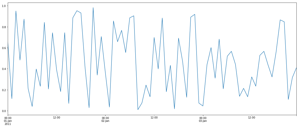
# Change frequency.
converted = ts.asfreq("45Min")
converted.head(10)
2011-01-01 00:00:00 0.653590
2011-01-01 00:45:00 NaN
2011-01-01 01:30:00 NaN
2011-01-01 02:15:00 NaN
2011-01-01 03:00:00 0.482191
2011-01-01 03:45:00 NaN
2011-01-01 04:30:00 NaN
2011-01-01 05:15:00 NaN
2011-01-01 06:00:00 0.040710
2011-01-01 06:45:00 NaN
Freq: 45T, dtype: float64# Change frequency and fill gaps.
# ffill: fills forward the nans (causal).
converted = ts.asfreq("45Min", method="ffill")
converted.head(10)2011-01-01 00:00:00 0.653590
2011-01-01 00:45:00 0.653590
2011-01-01 01:30:00 0.115007
2011-01-01 02:15:00 0.950283
2011-01-01 03:00:00 0.482191
2011-01-01 03:45:00 0.482191
2011-01-01 04:30:00 0.872475
2011-01-01 05:15:00 0.212333
2011-01-01 06:00:00 0.040710
2011-01-01 06:45:00 0.040710
Freq: 45T, dtype: float64# Resample daily using mean() to aggregate.
ts.resample("D").mean()2011-01-01 0.515735
2011-01-02 0.469341
2011-01-03 0.408907
Freq: D, dtype: float64ts.plot(label="ts")
converted.plot(label="converted")
ts.resample("D").mean().plot(label="daily mean")
plt.legend(loc="best")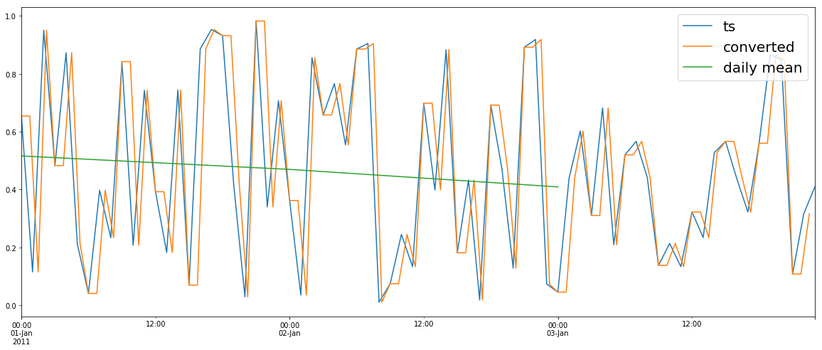
Time stamps vs time spans
http://
Timestamp = represents a single point in time
- create with: to_datetime(), Timestamp()
DatetimeIndex = index of Timestamp
- create with: to_datetime(), date_range(), DatetimeIndex()
Period = represents a single time span
- create with: Period()
PeriodIndex = index of Period
- create with: period_range(), PeriodIndex()
pd.Timestamp(datetime.datetime(2012, 5, 1))Timestamp('2012-05-01 00:00:00')pd.Timestamp("2012-05-01")Timestamp('2012-05-01 00:00:00')pd.Timestamp(2012, 5, 1)Timestamp('2012-05-01 00:00:00')pd.Period("2011-01", freq="D")Period('2011-01-01', 'D')# Timestamp is coerced to DatetimeIndex when used as index in DataFrame and Series.
dates = [pd.Timestamp(d) for d in "2015-05-01 2015-05-02 2015-05-03".split()]
np.random.seed(1000)
ts = pd.Series(np.random.randn(len(dates)), dates)
print("ts=", ts)
print("type(ts.index)=", type(ts.index))
# Note that there is no frequency inferred.
print("ts.index=", ts.index)ts= 2015-05-01 -0.804458
2015-05-02 0.320932
2015-05-03 -0.025483
dtype: float64
type(ts.index)= <class 'pandas.core.indexes.datetimes.DatetimeIndex'>
ts.index= DatetimeIndex(['2015-05-01', '2015-05-02', '2015-05-03'], dtype='datetime64[ns]', freq=None)
# Extract a np.array of datetime.date.
ts.index.date
array([datetime.date(2015, 5, 1), datetime.date(2015, 5, 2),
datetime.date(2015, 5, 3)], dtype=object)# Period is coerced to PeriodIndex.
periods = [pd.Period(d) for d in "2012-01 2012-02 2012-03".split()]
ts = pd.Series(np.random.randn(len(periods)), periods)
print("ts=", ts)
print("type(ts.index)=", type(ts.index))
# Note that a month frequency is inferred.
print("ts.index=", ts.index)ts= 2012-01 0.644324
2012-02 -0.300797
2012-03 0.389475
Freq: M, dtype: float64
type(ts.index)= <class 'pandas.core.indexes.period.PeriodIndex'>
ts.index= PeriodIndex(['2012-01', '2012-02', '2012-03'], dtype='period[M]', freq='M')
to_datetime()
http://
- Used to convert to pd.Timestamp objects
# Series with a bunch of strings (objects).
srs = pd.Series(["Jul 31, 2009", "2010-01-10", None])
print("srs=", srs)

# Convert to string with timestamps.
print(pd.to_datetime(srs))
srs= 0 Jul 31, 2009
1 2010-01-10
2 None
dtype: object
0 2009-07-31
1 2010-01-10
2 NaT
dtype: datetime64[ns]
# pd.to_datetime() returns a list or a single element.
print(pd.to_datetime("2010-11-12"))
print(pd.to_datetime(["2010-11-12", "2010-11-13", "2010-11-14"]))
2010-11-12 00:00:00
DatetimeIndex(['2010-11-12', '2010-11-13', '2010-11-14'], dtype='datetime64[ns]', freq=None)
# Using Epochs.
pd.to_datetime(
    [1349720105, 1349806505, 1349892905, 1349979305, 1350065705], unit="s"
)
DatetimeIndex(['2012-10-08 18:15:05', '2012-10-09 18:15:05', '2012-10-10 18:15:05', '2012-10-11 18:15:05', '2012-10-12 18:15:05'], dtype='datetime64[ns]', freq=None)pd.to_datetime(
[
dt * 1000
for dt in [1349720105, 1349806505, 1349892905, 1349979305, 1350065705]
],
unit="ms",
)DatetimeIndex(['2012-10-08 18:15:05', '2012-10-09 18:15:05', '2012-10-10 18:15:05', '2012-10-11 18:15:05', '2012-10-12 18:15:05'], dtype='datetime64[ns]', freq=None)# ??? Not working in 0.19
if False:
dts = pd.to_datetime(["2010-11-12", "2010-11-13", "2010-11-14"])
pd.to_pydatetime(dts)date_range()
http://
- date_range() is used to generate ranges of Timestamps
- date_range() is inclusive
# Beginning of month (MS=month start).
idx = pd.date_range("2000-1-1", periods=10, freq="MS")
idx
DatetimeIndex(['2000-01-01', '2000-02-01', '2000-03-01', '2000-04-01', '2000-05-01', '2000-06-01', '2000-07-01', '2000-08-01', '2000-09-01', '2000-10-01'], dtype='datetime64[ns]', freq='MS')# End of month.
idx = pd.date_range("2000-1-1", periods=10, freq="M")
idxDatetimeIndex(['2000-01-31', '2000-02-29', '2000-03-31', '2000-04-30', '2000-05-31', '2000-06-30', '2000-07-31', '2000-08-31', '2000-09-30', '2000-10-31'], dtype='datetime64[ns]', freq='M')# All (calendar) days.
idx = pd.date_range("2000-1-1", periods=10, freq="D")
idxDatetimeIndex(['2000-01-01', '2000-01-02', '2000-01-03', '2000-01-04', '2000-01-05', '2000-01-06', '2000-01-07', '2000-01-08', '2000-01-09', '2000-01-10'], dtype='datetime64[ns]', freq='D')# All business days.
idx = pd.bdate_range("2000-1-1", periods=1000)
idxDatetimeIndex(['2000-01-03', '2000-01-04', '2000-01-05', '2000-01-06', '2000-01-07', '2000-01-10', '2000-01-11', '2000-01-12', '2000-01-13', '2000-01-14',
...
'2003-10-20', '2003-10-21', '2003-10-22', '2003-10-23', '2003-10-24', '2003-10-27', '2003-10-28', '2003-10-29', '2003-10-30', '2003-10-31'], dtype='datetime64[ns]', length=1000, freq='B')# Specify [start, end].
start = datetime.datetime(2011, 1, 1)
end = datetime.datetime(2012, 1, 1)
idx = pd.date_range(start, end)
idxDatetimeIndex(['2011-01-01', '2011-01-02', '2011-01-03', '2011-01-04', '2011-01-05', '2011-01-06', '2011-01-07', '2011-01-08', '2011-01-09', '2011-01-10',
...
'2011-12-23', '2011-12-24', '2011-12-25', '2011-12-26', '2011-12-27', '2011-12-28', '2011-12-29', '2011-12-30', '2011-12-31', '2012-01-01'], dtype='datetime64[ns]', length=366, freq='D')# Beginning of month.
pd.date_range(start, end, freq="MS")DatetimeIndex(['2011-01-01', '2011-02-01', '2011-03-01', '2011-04-01', '2011-05-01', '2011-06-01', '2011-07-01', '2011-08-01', '2011-09-01', '2011-10-01', '2011-11-01', '2011-12-01', '2012-01-01'], dtype='datetime64[ns]', freq='MS')# Every week (starting from Sunday).
pd.date_range(start, end, freq="W")DatetimeIndex(['2011-01-02', '2011-01-09', '2011-01-16', '2011-01-23', '2011-01-30', '2011-02-06', '2011-02-13', '2011-02-20', '2011-02-27', '2011-03-06', '2011-03-13', '2011-03-20', '2011-03-27', '2011-04-03', '2011-04-10', '2011-04-17', '2011-04-24', '2011-05-01', '2011-05-08', '2011-05-15', '2011-05-22', '2011-05-29', '2011-06-05', '2011-06-12', '2011-06-19', '2011-06-26', '2011-07-03', '2011-07-10', '2011-07-17', '2011-07-24', '2011-07-31', '2011-08-07', '2011-08-14', '2011-08-21', '2011-08-28', '2011-09-04', '2011-09-11', '2011-09-18', '2011-09-25', '2011-10-02', '2011-10-09', '2011-10-16', '2011-10-23', '2011-10-30', '2011-11-06', '2011-11-13', '2011-11-20', '2011-11-27', '2011-12-04', '2011-12-11', '2011-12-18', '2011-12-25', '2012-01-01'], dtype='datetime64[ns]', freq='W-SUN')print(pd.to_datetime("2011-01-02").dayofweek)6
# Start from beginning for 20 business days.
pd.bdate_range(start=start, periods=20)
DatetimeIndex(['2011-01-03', '2011-01-04', '2011-01-05', '2011-01-06', '2011-01-07', '2011-01-10', '2011-01-11', '2011-01-12', '2011-01-13', '2011-01-14', '2011-01-17', '2011-01-18', '2011-01-19', '2011-01-20', '2011-01-21', '2011-01-24', '2011-01-25', '2011-01-26', '2011-01-27', '2011-01-28'], dtype='datetime64[ns]', freq='B')# Start from end for 20 business days.
pd.bdate_range(end=end, periods=20)DatetimeIndex(['2011-12-05', '2011-12-06', '2011-12-07', '2011-12-08', '2011-12-09', '2011-12-12', '2011-12-13', '2011-12-14', '2011-12-15', '2011-12-16', '2011-12-19', '2011-12-20', '2011-12-21', '2011-12-22', '2011-12-23', '2011-12-26', '2011-12-27', '2011-12-28', '2011-12-29', '2011-12-30'], dtype='datetime64[ns]', freq='B')DatetimeIndex
http://
- DatetimeIndex is index of pandas objects
- It supports union / intersection operations, shifting operations
# Build a df with an index every last day of the month.
idx = pd.date_range(start, end, freq="BM")
ts = pd.Series(np.random.randn(len(idx)), index=idx)
ts.index
DatetimeIndex(['2011-01-31', '2011-02-28', '2011-03-31', '2011-04-29', '2011-05-31', '2011-06-30', '2011-07-29', '2011-08-31', '2011-09-30', '2011-10-31', '2011-11-30', '2011-12-30'], dtype='datetime64[ns]', freq='BM')ts[:5].indexDatetimeIndex(['2011-01-31', '2011-02-28', '2011-03-31', '2011-04-29', '2011-05-31'], dtype='datetime64[ns]', freq='BM')# Skip 2.
ts[::2].indexDatetimeIndex(['2011-01-31', '2011-03-31', '2011-05-31', '2011-07-29', '2011-09-30', '2011-11-30'], dtype='datetime64[ns]', freq='2BM')# Index with string representing a date.
ts["1/31/2011"]-0.10743730169089667# Index with datetime.
ts[datetime.date(2011, 1, 31)]-0.10743730169089667# Slice with string.
ts["2011-12-25":]2011-12-30 0.705692
Freq: BM, dtype: float64# Slice with datetime().
ts[datetime.datetime(2011, 12, 25) :]2011-12-30 0.705692
Freq: BM, dtype: float64# Slice with partial string.
ts["2011"]2011-01-31 -0.107437
2011-02-28 -0.479983
2011-03-31 0.595036
2011-04-29 -0.464668
2011-05-31 0.667281
2011-06-30 -0.806116
2011-07-29 -1.196070
2011-08-31 -0.405960
2011-09-30 -0.182377
2011-10-31 0.103193
2011-11-30 -0.138422
2011-12-30    0.705692
Freq: BM, dtype: float64
# Select with partial string.
ts["2011-06"]2011-06-30 -0.806116
Freq: BM, dtype: float64# Label slicing implies that endpoints are included
# (different from python convention, but same as np).
ts["2011-01-31":"2011-03-31"]2011-01-31 -0.107437
2011-02-28 -0.479983
2011-03-31 0.595036
Freq: BM, dtype: float64# truncate() is equivalent to slicing (both endpoints are included in the sliced object).
ts.truncate(before="10/31/2011", after="12/31/2011")2011-10-31 0.103193
2011-11-30 -0.138422
2011-12-30    0.705692
Freq: BM, dtype: float64Time/date components.
http://
dt = pd.Timestamp("2012-05-01")
print(type(dt), dt)

dt = pd.to_datetime("2012-05-01")
print(type(dt), dt)
<class 'pandas._libs.tslib.Timestamp'> 2012-05-01 00:00:00
<class 'pandas._libs.tslib.Timestamp'> 2012-05-01 00:00:00
dt = pd.Timestamp("2012-05-01")

print("year=", dt.year)
print("microsecond=", dt.microsecond)
print("date=", dt.date())
print("dayofyear=", dt.dayofyear)
print("weekofyear=", dt.weekofyear)
print("week=", dt.week)
print("dayofweek=", dt.dayofweek)
print("weekday=", dt.weekday())
print("weekday_name=", dt.weekday_name)
# Number of days in the month of dt.
print("days_in_month=", dt.days_in_month)
print("is_month_start=", dt.is_month_start)
print("is_month_end=", dt.is_month_end)
print("is_leap_year=", dt.is_leap_year)
year= 2012
microsecond= 0
date= 2012-05-01
dayofyear= 122
weekofyear= 18
week= 18
dayofweek= 1
weekday= 1
weekday_name= Tuesday
days_in_month= 31
is_month_start= True
is_month_end= False
is_leap_year= True
Offset objects.
http://
Frequency strings (e.g., M, W, BM) are converted to pandas pd.offsets.DateOffset(), which represents a regular frequency increment
DateOffset() keeps results as Timestamp (differently from timedelta)
Offset information are at
# Using pd.offsets.DateOffset() returns a Timestamp.
d = datetime.datetime(2008, 8, 18, 19, 0)
print(type(d), d)

next_d = d + pd.offsets.DateOffset(months=4, days=5)
print(type(next_d), next_d)
<type 'datetime.datetime'> 2008-08-18 19:00:00
<class 'pandas._libs.tslib.Timestamp'> 2008-12-23 19:00:00
print("BDay=", d + pd.offsets.BDay())
print("Week=", d + pd.offsets.Week())
# print "WeekOfMonth=", d + pd.offsets.WeekOfMonth()
BDay= 2008-08-19 19:00:00
Week= 2008-08-25 19:00:00
# Use DateOffset() to align to month.
print("d=", d)
print("MonthEnd=", d + pd.offsets.MonthEnd())
print("MonthBegin=", d + pd.offsets.MonthBegin())

# Align to first / last business day.
print("BMonthEnd=", d + pd.offsets.BMonthEnd())
print("BMonthBegin=", d + pd.offsets.BMonthBegin())
d= 2008-08-18 19:00:00
MonthEnd= 2008-08-31 19:00:00
MonthBegin= 2008-09-01 19:00:00
BMonthEnd= 2008-08-29 19:00:00
BMonthBegin= 2008-09-01 19:00:00
# Offset can be manipulated with arithmetic.
offset = 5 * pd.offsets.BDay()
print(type(offset))
print(offset)
<class 'pandas.tseries.offsets.BusinessDay'>
<5 * BusinessDays>
# Some offsets can be parametrized.
print(d)

# Preserve the hour.
print(d + pd.offsets.Week())

# Align to a specific day of the week
print(d + pd.offsets.Week(weekday=4))
print((d + pd.offsets.Week(weekday=4)).dayofweek)

# This aligns to midnight.
print(d + pd.offsets.Week(normalize=True))
2008-08-18 19:00:00
2008-08-25 19:00:00
2008-08-22 19:00:00
4
2008-08-25 00:00:00
# Offsets also works with Series / DataFrames (although might be slow since it is not vectorized).
rng = pd.date_range(start="2012-01-01", end="2012-01-03", freq="1D")
s = pd.Series(rng)
print(s)

print(s + pd.offsets.DateOffset(months=1))
0 2012-01-01
1 2012-01-02
2 2012-01-03
dtype: datetime64[ns]
0 2012-02-01
1 2012-02-02
2 2012-02-03
dtype: datetime64[ns]
# In general string aliases and offset objects are interchangeable.
print(pd.date_range(start="2012-01-01", end="2012-01-10", freq="3D"))
print(
    pd.date_range(
        start="2012-01-01", end="2012-01-10", freq=3 * pd.offsets.Day()
    )
)
DatetimeIndex(['2012-01-01', '2012-01-04', '2012-01-07', '2012-01-10'], dtype='datetime64[ns]', freq='3D')
DatetimeIndex(['2012-01-01', '2012-01-04', '2012-01-07', '2012-01-10'], dtype='datetime64[ns]', freq='3D')
# One can combine day and intraday offsets in string offsets.
pd.date_range(start, periods=10, freq="2h20min")
DatetimeIndex(['2011-01-01 00:00:00', '2011-01-01 02:20:00', '2011-01-01 04:40:00', '2011-01-01 07:00:00', '2011-01-01 09:20:00', '2011-01-01 11:40:00', '2011-01-01 14:00:00', '2011-01-01 16:20:00', '2011-01-01 18:40:00', '2011-01-01 21:00:00'], dtype='datetime64[ns]', freq='140T')Time series-related operations
idx = pd.date_range(start="2012-01-01", end="2012-01-07", freq="1D")
ts = pd.Series(list(range(len(idx))), index=idx)
ts
2012-01-01 0
2012-01-02 1
2012-01-03 2
2012-01-04 3
2012-01-05 4
2012-01-06 5
2012-01-07 6
Freq: D, dtype: int64# Shift back, i.e., yesterday becomes today.
# shift() doesn't change the time scale.
ts.shift(1)2012-01-01 NaN
2012-01-02 0.0
2012-01-03 1.0
2012-01-04 2.0
2012-01-05 3.0
2012-01-06 4.0
2012-01-07 5.0
Freq: D, dtype: float64# By specifying a freq one can shift the time series, by shifting the time scale.
# Note that the first element is not NA since the data is not being realigned.
# ??? Weird that there are two 2012-01-09 now...
ts.shift(1, freq=pd.offsets.BDay())2012-01-02 0
2012-01-03 1
2012-01-04 2
2012-01-05 3
2012-01-06 4
2012-01-09 5
2012-01-09 6
dtype: int64Frequency conversion
http://
- asfreq() allows to change frequency of a time series.
- in practice it is equivalent to a call to date_range() and a call to reindex()
np.random.seed(1000)
idx = pd.date_range("1/1/2010", periods=3, freq=3 * pd.offsets.BDay())
ts = pd.Series(np.random.randn(len(idx)), index=idx)

ts
2010-01-01 -0.804458
2010-01-06 0.320932
2010-01-11 -0.025483
Freq: 3B, dtype: float64# Sample using calendar days.
ts.asfreq(pd.offsets.Day())2010-01-01 -0.804458
2010-01-02 NaN
2010-01-03 NaN
2010-01-04 NaN
2010-01-05 NaN
2010-01-06 0.320932
2010-01-07 NaN
2010-01-08 NaN
2010-01-09 NaN
2010-01-10 NaN
2010-01-11 -0.025483
Freq: D, dtype: float64# Sample using business days.
ts.asfreq(pd.offsets.BDay())2010-01-01 -0.804458
2010-01-04 NaN
2010-01-05 NaN
2010-01-06 0.320932
2010-01-07 NaN
2010-01-08 NaN
2010-01-11 -0.025483
Freq: B, dtype: float64ts.asfreq(pd.offsets.BDay(), method="ffill")2010-01-01 -0.804458
2010-01-04 -0.804458
2010-01-05 -0.804458
2010-01-06 0.320932
2010-01-07 0.320932
2010-01-08 0.320932
2010-01-11 -0.025483
Freq: B, dtype: float64Time span representation
http://
- Period() represents a span of time
- Regular intervals of time are represented by Period objects
# Arithmetic operations on periods.
p = pd.Period("2012-1-1", freq="D")
print(type(p), p)
print(p + 1)
print(p - 3)
<class 'pandas._libs.period.Period'> 2012-01-01
2012-01-02
2011-12-29
p = pd.Timestamp("2012-1-1", freq="D")
print(type(p), p)
print(p + 1)
print(p - 3)
<class 'pandas._libs.tslib.Timestamp'> 2012-01-01 00:00:00
2012-01-02 00:00:00
2011-12-29 00:00:00
prng = pd.period_range("1/1/2011", "1/1/2012", freq="M")
prng
PeriodIndex(['2011-01', '2011-02', '2011-03', '2011-04', '2011-05', '2011-06', '2011-07', '2011-08', '2011-09', '2011-10', '2011-11', '2011-12', '2012-01'], dtype='period[M]', freq='M')np.random.seed(1000)
ts = pd.Series(np)Time zone handling
# By default pandas objects are time zone unaware.
rng = pd.date_range("3/6/2012 00:00", periods=15, freq="D")
print(rng)
print(rng.tz is None)
DatetimeIndex(['2012-03-06', '2012-03-07', '2012-03-08', '2012-03-09', '2012-03-10', '2012-03-11', '2012-03-12', '2012-03-13', '2012-03-14', '2012-03-15', '2012-03-16', '2012-03-17', '2012-03-18', '2012-03-19', '2012-03-20'], dtype='datetime64[ns]', freq='D')
True
# Using pandas timezone support.
rng = pd.date_range("3/6/2012 00:00", periods=10, freq="D", tz="Europe/London")
print(rng)
print(rng.tz is None)
print(rng.tz)
DatetimeIndex(['2012-03-06', '2012-03-07', '2012-03-08', '2012-03-09', '2012-03-10', '2012-03-11', '2012-03-12', '2012-03-13', '2012-03-14', '2012-03-15'], dtype='datetime64[ns, Europe/London]', freq='D')
False
Europe/London
# Using pytz timezone.
import pytz

pytz_ = pytz.timezone("Europe/London")
rng_pytz = pd.date_range("3/6/2012 00:00", periods=10, freq="D", tz=pytz_)
print(rng_pytz)
DatetimeIndex(['2012-03-06', '2012-03-07', '2012-03-08', '2012-03-09', '2012-03-10', '2012-03-11', '2012-03-12', '2012-03-13', '2012-03-14', '2012-03-15'], dtype='datetime64[ns, Europe/London]', freq='D')
# tz_localize() just forces a tz-unaware datetime to become aware of
# the passed tz. It's up to the caller to know how to interpret the
# date time.
# datetime() doesn't have tz_localize method.
dt = pd.to_datetime(datetime.date(2000, 2, 1))
print("dt=", type(dt), dt)

# datetime() doesn't have tz_localize method.
print("dt=", type(dt), dt.tz_localize("US/Eastern"))
dt= <class 'pandas._libs.tslib.Timestamp'> 2000-02-01 00:00:00
dt= <class 'pandas._libs.tslib.Timestamp'> 2000-02-01 00:00:00-05:00
# Once a datetime is localized, one can represent the same data with
# different timezones.
dt = pd.to_datetime(datetime.date(2000, 2, 1))
print("dt=", type(dt), dt)

dt = dt.tz_localize("UTC")
print("dt=", type(dt), dt)

dt = dt.tz_convert("US/Eastern")
print("dt=", type(dt), dt)
dt= <class 'pandas._libs.tslib.Timestamp'> 2000-02-01 00:00:00
dt= <class 'pandas._libs.tslib.Timestamp'> 2000-02-01 00:00:00+00:00
dt= <class 'pandas._libs.tslib.Timestamp'> 2000-01-31 19:00:00-05:00
# Localize and convert to timezone aware.
np.random.seed(1000)
rng = pd.date_range("3/6/2012 00:00", periods=15, freq="D")
ts = pd.Series(np.random.randn(len(rng)), rng)
print(ts.head(3))

ts_utc = ts.tz_localize("UTC")
print("\n", ts_utc.head(3))

print("\n", ts_utc.tz_convert("US/Eastern").head(3))
2012-03-06 -0.804458
2012-03-07 0.320932
2012-03-08 -0.025483
Freq: D, dtype: float64
2012-03-06 00:00:00+00:00 -0.804458
2012-03-07 00:00:00+00:00 0.320932
2012-03-08 00:00:00+00:00 -0.025483
Freq: D, dtype: float64
2012-03-05 19:00:00-05:00 -0.804458
2012-03-06 19:00:00-05:00 0.320932
2012-03-07 19:00:00-05:00 -0.025483
Freq: D, dtype: float64
# To remove localization.
ts_utc.tz_localize(None).head(3)
2012-03-06 -0.804458
2012-03-07 0.320932
2012-03-08 -0.025483
Freq: D, dtype: float64