Import
Import
import datetime

import numpy as np
import pandas as pd

%load_ext autoreload
%autoreload 2

%matplotlib inline
import notebook_utils
notebook_utils.notebook_config()
# matplotlib.rcParams["figure.figsize"] = (15, 6)numpy= 1.16.4
pandas= 0.25.0
matplotlib= 3.1.1
sklearn= 0.21.3
from notebook_utils import display_df

from IPython.display import displayGrouping
- groupby = split + apply + combine
np.random.seed(10)
df = pd.DataFrame(
    {
        "A": ["foo", "bar", "foo", "bar", "foo", "bar", "foo", "foo"],
        "B": ["one", "one", "two", "three", "two", "two", "one", "three"],
        "C": np.random.randn(8),
        "D": np.random.randn(8),
    }
)
df
Loading...
grouped = df.groupby("A")

print("keys=", list(grouped.groups.keys()))

display_df(grouped.get_group("foo"))
keys= ['foo', 'bar']
Loading...
Grouping series
idx = [1, 2, 3, 1, 2, 3]
s = pd.Series([1, 2, 3, 10, 20, 30], idx)
s
1 1
2 2
3 3
1 10
2 20
3 30
dtype: int64# groupby() by index values.
grouped = s.groupby(level=0)
print("keys=", list(grouped.groups.keys()))
print("first=\n", grouped.first())
print("last=\n", grouped.last())keys= [1, 2, 3]
first=
1 1
2 2
3 3
dtype: int64
last=
1 10
2 20
3 30
dtype: int64
Grouping df
df2 = pd.DataFrame({"X": ["B", "B", "A", "A"], "Y": [1, 2, 3, 4]})
df2
Loading...
# Note that groupby() sorts the group keys.
df2.groupby(["X"]).sum()
Loading...
# Observations are kept sorted within each group according to the original df.
df2.groupby("X").get_group("A")
Loading...
# Get a single group.
df2.groupby("X").get_group("B")
Loading...
# Get all groups and mapping.
df2.groupby("X").groups
{'A': Int64Index([2, 3], dtype='int64'),
'B': Int64Index([0, 1], dtype='int64')}# Group on two columns.
df2.groupby(["X", "Y"]).groups{('A', 3): Int64Index([2], dtype='int64'),
('A', 4): Int64Index([3], dtype='int64'),
('B', 1): Int64Index([0], dtype='int64'),
('B', 2): Int64Index([1], dtype='int64')}# Iterate over groups.
grouped = df2.groupby("X")
for name, group in grouped:
print("\nname=", name)
print(group)
name= A
   X  Y
2  A  3
3  A  4

name= B
   X  Y
0  B  1
1  B  2
Groupby + select
df_buyer = pd.DataFrame(
    {
        "Branch": "A A A A A A A B".split(),
        "Buyer": "Carl Mark Carl Carl Joe Joe Joe Carl".split(),
        "Quantity": [1, 3, 5, 1, 8, 1, 9, 3],
        "Date": [
            datetime.datetime(2013, 1, 1, 13, 0),
            datetime.datetime(2013, 1, 1, 13, 5),
            datetime.datetime(2013, 10, 1, 20, 0),
            datetime.datetime(2013, 10, 2, 10, 0),
            datetime.datetime(2013, 10, 1, 20, 0),
            datetime.datetime(2013, 10, 2, 10, 0),
            datetime.datetime(2013, 12, 2, 12, 0),
            datetime.datetime(2013, 12, 2, 14, 0),
        ],
    }
)

df_buyer
Loading...
# Group, transform, concat.
df_buyer.groupby("Buyer").head(1)
Loading...
# Group, transform, concat.
df_buyer.groupby("Buyer").head(2)
Loading...
df_buyer.groupby("Buyer").nth(2)Loading...
Groupby + plot.
_ = df_buyer.groupby("Buyer").boxplot()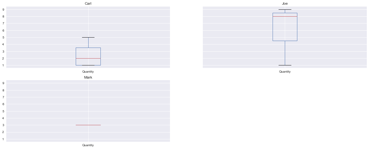
Groupby + aggregation
# Group and then aggregate groups with generic function.
display_df(grouped.aggregate(np.sum))
# print grouped.agg(np.sum)
Loading...
# Use pandas function.
grouped.sum()
Loading...
df.groupby(["A", "B"]).sum()Loading...
# Group-by, accumulate, and then convert multi-index into a regular column (opposite of set_index()).
df.groupby(["A", "B"]).sum().reset_index()
Loading...
# Since size() generates a single columns, the result is a multi-index series, instead of a df.
df.groupby(["A", "B"]).size()
A B
bar one 1
three 1
two 1
foo one 2
three 1
two 2
dtype: int64# Apply multiple functions to each group, producing hierarchical columns.
df.groupby("A").agg([np.sum, np.mean, np.std])Loading...
# Use names from dict for columns.
# It doesn't seem to work.
if False:
    df.groupby("A").agg({"sum_": np.sum, "mean_": np.mean, "std_": np.std})
groupby + transform.
- transform() returns an object that is indexed in the same way as the original one
- so groupby() + transform(), applies a function to each group.
np.random.seed(5)
index = pd.date_range("10/1/1999", periods=1100)
ts = pd.Series(np.random.normal(0.05, 2, 1100), index)
ts.cumsum().plot()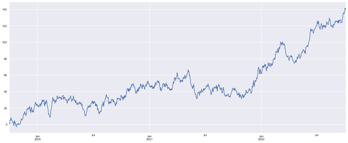
# Iterate by year.
sorted(ts.groupby(lambda x: x.year).groups.keys())
[1999, 2000, 2001, 2002]# This is an object computing a rolling window on the data.
rolling = ts.rolling(window=100, min_periods=100)
print(type(rolling))<class 'pandas.core.window.Rolling'>
# Compute a rolling window and apply mean: i.e., a rolling mean.
ts2 = rolling.mean()
ts2.plot()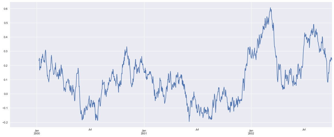
# Group by year.
key = lambda x: x.year
grouped = ts2.groupby(key)

# Transform each group by zscoring within the group.
zscore = lambda x: (x - x.mean()) / x.std()
transformed = grouped.transform(zscore)
transformed.plot()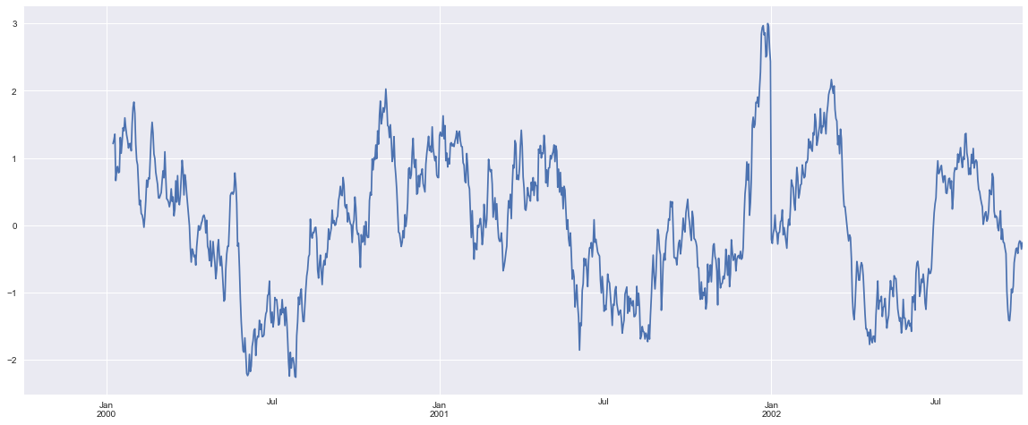
dfLoading...
if False:

    def print_(x):
        print("\n", x)

    df.groupby("A").transform(print_)
Apply rolling function generating multiple values.
np.random.seed(0)
df = pd.DataFrame(np.random.rand(100, 1))
f = lambda df: df.mean()
# res = pd.rolling_apply(df, 3, f, min_periods=3)
res = df.rolling(min_periods=3, window=3).apply(f)
res.head(10)
Loading...
df = pd.DataFrame(np.random.rand(100, 1))
# f = lambda df: [df.mean(), df.std()]
f = lambda df: df.mean()
# res = pd.rolling_apply(df, 3, f, min_periods=3)
res = df.rolling(min_periods=3, window=3).apply(f)
res.head(10)
Loading...
# It doesn't seem to work forgroupby + filter
- We filter a groupby based on their value
sf = pd.Series([1, 1, 2, 3, 3, 3])
print(sf.groupby(sf).groups)
{1: Int64Index([0, 1], dtype='int64'), 2: Int64Index([2], dtype='int64'), 3: Int64Index([3, 4, 5], dtype='int64')}
# Filter groupby by picking only groups with a sum larger.
sf.groupby(sf).filter(lambda x: x.sum() > 2)
3 3
4 3
5 3
dtype: int64Groupby + apply
- apply() can act as a reducer, transformer or filter
np.random.seed(10)
df = pd.DataFrame(
    {
        "A": ["foo", "bar", "foo", "bar", "foo", "bar", "foo", "foo"],
        "B": ["one", "one", "two", "three", "two", "two", "one", "three"],
        "C": np.random.randn(8),
        "D": np.random.randn(8),
    }
)
df
Loading...
dfLoading...
# Apply calls describe on each group and concat the results.
df.groupby("A").apply(lambda x: x.describe())
Loading...
Grouper
- If one needs more control of grouping, an object pd.Grouper can be used.
df_buyer = pd.DataFrame(
    {
        "Branch": "A A A A A A A B".split(),
        "Buyer": "Carl Mark Carl Carl Joe Joe Joe Carl".split(),
        "Quantity": [1, 3, 5, 1, 8, 1, 9, 3],
        "Date": [
            datetime.datetime(2013, 1, 1, 13, 0),
            datetime.datetime(2013, 1, 1, 13, 5),
            datetime.datetime(2013, 10, 1, 20, 0),
            datetime.datetime(2013, 10, 2, 10, 0),
            datetime.datetime(2013, 10, 1, 20, 0),
            datetime.datetime(2013, 10, 2, 10, 0),
            datetime.datetime(2013, 12, 2, 12, 0),
            datetime.datetime(2013, 12, 2, 14, 0),
        ],
    }
)

df_buyer
Loading...
# This is like resampling.
grouper = pd.Grouper(freq="1M", key="Date")

df_tmp = df_buyer.groupby(grouper).sum().dropna()
df_tmp
Loading...
df_tmp2 = df_tmp.copy()
df_tmp2.index += pd.offsets.MonthEnd(1)
df_tmp2
Loading...
TODO: finish
Downsampling with resample()
- resample() is conceptually a time-based groupby() followed by a transformation on each group
- downsample and use reduction method
- upsample and interpolate / fill values
# Build a df with 100 seconds worth of (random) data.
np.random.seed(1000)
rng = pd.date_range("1/1/2012", periods=100, freq="S")
ts0 = pd.Series(np.random.randint(0, 500, len(rng)), index=rng)
print(ts0.head())
print(ts0.tail())
2012-01-01 00:00:00 435
2012-01-01 00:00:01 87
2012-01-01 00:00:02 71
2012-01-01 00:00:03 192
2012-01-01 00:00:04 251
Freq: S, dtype: int64
2012-01-01 00:01:35 307
2012-01-01 00:01:36 437
2012-01-01 00:01:37 47
2012-01-01 00:01:38 56
2012-01-01 00:01:39 20
Freq: S, dtype: int64
# Summarize in 1 minute intervals.
ts0.resample("1Min").sum()
2012-01-01 00:00:00 16031
2012-01-01 00:01:00 8297
Freq: T, dtype: int64ts0.resample("1Min").max()2012-01-01 00:00:00 498
2012-01-01 00:01:00 471
Freq: T, dtype: int64# 'label' and 'loffset' can be used to manipulate the labels used to mark the intervals.
print(ts0.resample("1Min", label="right").mean())
print(ts0.resample("1Min", label="left").mean())
print(ts0.resample("1Min", label="left", loffset="1s").mean())2012-01-01 00:01:00 267.183333
2012-01-01 00:02:00 207.425000
Freq: T, dtype: float64
2012-01-01 00:00:00 267.183333
2012-01-01 00:01:00 207.425000
Freq: T, dtype: float64
2012-01-01 00:00:01 267.183333
2012-01-01 00:01:01 207.425000
dtype: float64
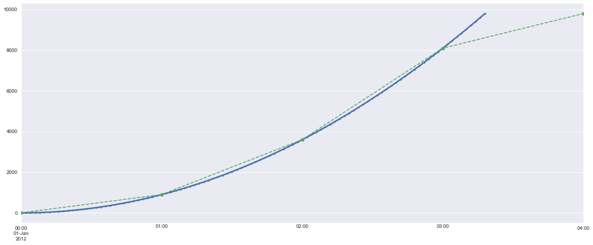
# Resample without summarizing.

# Build a df with 100 seconds worth of data.
np.random.seed(1000)
rng = pd.date_range("1/1/2012", periods=100, freq="2Min")
ts0_1 = pd.Series(np.arange(0, len(rng)) ** 2, index=rng)
ts0_1.plot(style=".-", lw=3)

# pandas 0.14 uses this syntax.
ts1_1 = ts0_1.resample("1H", how="last", closed="right", label="right")
ts1_1.plot(kind="line", style="o--")
/Users/gp/.conda/envs/jupyter/lib/python2.7/site-packages/ipykernel_launcher.py:10: FutureWarning: how in .resample() is deprecated
the new syntax is .resample(...).last()
# Remove the CWD from sys.path while we load stuff.
Upsampling with resample().
# Get a df with 2 seconds worth of data.
ts[:2]
1999-10-01 0.932455
1999-10-02 -0.611740
Freq: D, dtype: float64# 'closed' can be used to specify which end of the interval is closed.
# By default intervals are [a, b)
print(ts.resample("1Min").mean().head(10))
print(ts.resample("1Min", closed="left").mean().head(10))
# closed=right => (a, b]
print(ts.resample("1Min", closed="right").mean().head(10))1999-10-01 00:00:00 0.932455
1999-10-01 00:01:00 NaN
1999-10-01 00:02:00 NaN
1999-10-01 00:03:00 NaN
1999-10-01 00:04:00 NaN
1999-10-01 00:05:00 NaN
1999-10-01 00:06:00 NaN
1999-10-01 00:07:00 NaN
1999-10-01 00:08:00 NaN
1999-10-01 00:09:00 NaN
Freq: T, dtype: float64
1999-10-01 00:00:00 0.932455
1999-10-01 00:01:00 NaN
1999-10-01 00:02:00 NaN
1999-10-01 00:03:00 NaN
1999-10-01 00:04:00 NaN
1999-10-01 00:05:00 NaN
1999-10-01 00:06:00 NaN
1999-10-01 00:07:00 NaN
1999-10-01 00:08:00 NaN
1999-10-01 00:09:00 NaN
Freq: T, dtype: float64
1999-09-30 23:59:00 0.932455
1999-10-01 00:00:00 NaN
1999-10-01 00:01:00 NaN
1999-10-01 00:02:00 NaN
1999-10-01 00:03:00 NaN
1999-10-01 00:04:00 NaN
1999-10-01 00:05:00 NaN
1999-10-01 00:06:00 NaN
1999-10-01 00:07:00 NaN
1999-10-01 00:08:00 NaN
Freq: T, dtype: float64
# Resample from seconds to 250 millisecs.
# asfreq() is used to expand the resampler.
ts[:2].resample("250L").asfreq().head(10)
1999-10-01 00:00:00.000 0.932455
1999-10-01 00:00:00.250 NaN
1999-10-01 00:00:00.500 NaN
1999-10-01 00:00:00.750 NaN
1999-10-01 00:00:01.000 NaN
1999-10-01 00:00:01.250 NaN
1999-10-01 00:00:01.500 NaN
1999-10-01 00:00:01.750 NaN
1999-10-01 00:00:02.000 NaN
1999-10-01 00:00:02.250 NaN
Freq: 250L, dtype: float64ts[:2].resample("250L").ffill().head(10)1999-10-01 00:00:00.000 0.932455
1999-10-01 00:00:00.250 0.932455
1999-10-01 00:00:00.500 0.932455
1999-10-01 00:00:00.750 0.932455
1999-10-01 00:00:01.000 0.932455
1999-10-01 00:00:01.250 0.932455
1999-10-01 00:00:01.500 0.932455
1999-10-01 00:00:01.750 0.932455
1999-10-01 00:00:02.000 0.932455
1999-10-01 00:00:02.250 0.932455
Freq: 250L, dtype: float64ts[:2].resample("250L").ffill(limit=2).head(10)1999-10-01 00:00:00.000 0.932455
1999-10-01 00:00:00.250 0.932455
1999-10-01 00:00:00.500 0.932455
1999-10-01 00:00:00.750 NaN
1999-10-01 00:00:01.000 NaN
1999-10-01 00:00:01.250 NaN
1999-10-01 00:00:01.500 NaN
1999-10-01 00:00:01.750 NaN
1999-10-01 00:00:02.000 NaN
1999-10-01 00:00:02.250 NaN
Freq: 250L, dtype: float64Sparse resampling
sparse timeseries are ones with fewer points relative to the amount of time
rng = pd.date_range("2014-1-1", periods=100, freq="D")
rng += pd.Timedelta("1s")
print(rng[:5])
DatetimeIndex(['2014-01-01 00:00:01', '2014-01-02 00:00:01', '2014-01-03 00:00:01', '2014-01-04 00:00:01', '2014-01-05 00:00:01'], dtype='datetime64[ns]', freq='D')
ts3 = pd.Series(list(range(100)), index=rng)
ts3.head()
2014-01-01 00:00:01 0
2014-01-02 00:00:01 1
2014-01-03 00:00:01 2
2014-01-04 00:00:01 3
2014-01-05 00:00:01 4
Freq: D, dtype: int64# Upsample the daily ts every 3 mins, getting a very sparse time series.
ts4 = ts3.resample("3T").sum()ts4.indexDatetimeIndex(['2014-01-01 00:00:00', '2014-01-01 00:03:00', '2014-01-01 00:06:00', '2014-01-01 00:09:00', '2014-01-01 00:12:00', '2014-01-01 00:15:00', '2014-01-01 00:18:00', '2014-01-01 00:21:00', '2014-01-01 00:24:00', '2014-01-01 00:27:00',
...
'2014-04-09 23:33:00', '2014-04-09 23:36:00', '2014-04-09 23:39:00', '2014-04-09 23:42:00', '2014-04-09 23:45:00', '2014-04-09 23:48:00', '2014-04-09 23:51:00', '2014-04-09 23:54:00', '2014-04-09 23:57:00', '2014-04-10 00:00:00'], dtype='datetime64[ns]', length=47521, freq='3T')Resample starting from a given offset (e.g., minutes, hours, days)
# Get a data frame with 60 hours.
idx = pd.date_range("2012-01-01-17", freq="H", periods=60)
ts5 = pd.Series(data=[1] * 60, index=idx)
print(ts5.head())
print(ts5.tail())
2012-01-01 17:00:00 1
2012-01-01 18:00:00 1
2012-01-01 19:00:00 1
2012-01-01 20:00:00 1
2012-01-01 21:00:00 1
Freq: H, dtype: int64
2012-01-04 00:00:00 1
2012-01-04 01:00:00 1
2012-01-04 02:00:00 1
2012-01-04 03:00:00 1
2012-01-04 04:00:00 1
Freq: H, dtype: int64
ts5.resample("D").sum()2012-01-01 7
2012-01-02 24
2012-01-03 24
2012-01-04 5
Freq: D, dtype: int64# By specifying a period in hours and setting the initial hour, one can shift the sampling intervals.
ts5.resample("24H", base=17).sum()2012-01-01 17:00:00 24
2012-01-02 17:00:00 24
2012-01-03 17:00:00 12
Freq: 24H, dtype: int64# Resample daily starting from 7:45am (= 60 * 24 + 45 = 465).
ts5.resample("1440Min", base=465).sum()2012-01-01 07:45:00 15
2012-01-02 07:45:00 24
2012-01-03 07:45:00 21
Freq: 1440T, dtype: int64Resample dataframes.
http://
# Df with 1000 seconds worth of data and multiple columns.
np.random.seed(1000)
df = pd.DataFrame(
    np.random.randn(1000, 3),
    index=pd.date_range("1/1/2012", freq="S", periods=1000),
    columns="A B C".split(" "),
)
print(df.head(2))
print("...")
print(df.tail(2))
A B C
2012-01-01 00:00:00 -0.804458 0.320932 -0.025483
2012-01-01 00:00:01 0.644324 -0.300797 0.389475
...
A B C
2012-01-01 00:16:38 -0.363336 0.154937 0.909393
2012-01-01 00:16:39 -1.072566 -1.199570 0.223837
# Apply the same function to each column.
df.resample("3T").mean()
Loading...
# Specify custom function.
df.resample("3T").agg(lambda x: x.mean())
Loading...
# Apply function to only certain columns.
# NOTE: we tell the resampler which columns to resample instead of selecting columns first.
df.resample("3T")[["A", "B"]].mean()
Loading...
# Apply multiple functions to a single column.
df.resample("3T")["A"].agg([np.sum, np.mean, np.std])
Loading...
# Assign names to columns.
df.resample("3T")["A"].agg({"res1": np.sum, "res2": np.mean})
/Users/gp/.conda/envs/jupyter/lib/python2.7/site-packages/ipykernel_launcher.py:3: FutureWarning: using a dict on a Series for aggregation
is deprecated and will be removed in a future version
This is separate from the ipykernel package so we can avoid doing imports until
Loading...
# Apply multiple functions to each column, returning a hierarchical index.
df.resample("3T").agg([np.sum, np.mean])
Loading...
# Specify different multiple functions for each column, returning a hierarchical index.
df.resample("3T").agg({"A": [np.sum, np.mean], "B": [np.mean]})
Loading...
Resample with asfreq()
np.random.seed(1000)
idx = pd.date_range("1/1/2010", periods=10, freq=pd.offsets.BDay())
ts6 = pd.Series(np.random.rand(idx.shape[0]), index=idx)
ts6
2010-01-01 0.653590
2010-01-04 0.115007
2010-01-05 0.950283
2010-01-06 0.482191
2010-01-07 0.872475
2010-01-08 0.212333
2010-01-11 0.040710
2010-01-12 0.397194
2010-01-13 0.233132
2010-01-14 0.841741
Freq: B, dtype: float64# Resample using a certain frequency: from business days to calendar days.
ts6.asfreq(pd.offsets.Day())2010-01-01 0.653590
2010-01-02 NaN
2010-01-03 NaN
2010-01-04 0.115007
2010-01-05 0.950283
2010-01-06 0.482191
2010-01-07 0.872475
2010-01-08 0.212333
2010-01-09 NaN
2010-01-10 NaN
2010-01-11 0.040710
2010-01-12 0.397194
2010-01-13 0.233132
2010-01-14 0.841741
Freq: D, dtype: float64Resample using groupby().
# groupby using time intervals and compute a function for each group.
# Note that we keep all dates.
grouper = pd.TimeGrouper("1W")

ts6.groupby(grouper).transform(lambda x: x.mean())
2010-01-01 0.653590
2010-01-04 0.526458
2010-01-05 0.526458
2010-01-06 0.526458
2010-01-07 0.526458
2010-01-08 0.526458
2010-01-11 0.378194
2010-01-12 0.378194
2010-01-13 0.378194
2010-01-14 0.378194
Freq: B, dtype: float64TODO: finish
Reshaping
Reshaping by pivoting
# Data in "stacked" or "record" format.
# For each date and each variable there is an observation.
idx = pd.date_range(start="20010101", end="20010103").tolist() * 4
np.random.seed(1000)
df = pd.DataFrame(np.random.rand(len(idx), 1), columns="value".split())
df.insert(0, "date", idx)
df.insert(1, "variable", ["A"] * 3 + ["B"] * 3 + ["C"] * 3 + ["D"] * 3)
df.index.name = "date"
print(df)
date variable value
date
0 2001-01-01 A 0.653590
1 2001-01-02 A 0.115007
2 2001-01-03 A 0.950283
3 2001-01-01 B 0.482191
4 2001-01-02 B 0.872475
5 2001-01-03 B 0.212333
6 2001-01-01 C 0.040710
7 2001-01-02 C 0.397194
8 2001-01-03 C 0.233132
9 2001-01-01 D 0.841741
10 2001-01-02 D 0.207082
11 2001-01-03 D 0.742470
# Assume we are interested in observations for variable "A".
df[df["variable"] == "A"]
Loading...
# The index is date, the values in "variable" become columns, and the values in "value"
# become the values in the df.
df.pivot(index="date", columns="variable", values="value")
Loading...
# If there are more than one value (i.e., more type of observations for a variable)
# one gets multi-index columns.
df["value2"] = df["value"] * 2.0
print(df)

df.pivot(index="date", columns="variable")
date variable value value2
date
0 2001-01-01 A 0.653590 1.307179
1 2001-01-02 A 0.115007 0.230014
2 2001-01-03 A 0.950283 1.900566
3 2001-01-01 B 0.482191 0.964383
4 2001-01-02 B 0.872475 1.744949
5 2001-01-03 B 0.212333 0.424665
6 2001-01-01 C 0.040710 0.081419
7 2001-01-02 C 0.397194 0.794389
8 2001-01-03 C 0.233132 0.466264
9 2001-01-01 D 0.841741 1.683481
10 2001-01-02 D 0.207082 0.414165
11 2001-01-03 D 0.742470 1.484939
Loading...
Reshaping by stacking / unstacking
# zip(list1, list2) creates pairs iterating on the lists.
# In other words it iterates on the columns of the stacked versions of the lists,
# effectively transposing.
list(zip("a b c d".split(), "1 2 3 4".split()))
[('a', '1'), ('b', '2'), ('c', '3'), ('d', '4')]list(zip("a b c d".split(), "1 2 3 4".split(), "x y z w".split()))[('a', '1', 'x'), ('b', '2', 'y'), ('c', '3', 'z'), ('d', '4', 'w')]tuples = [("a", "1"), ("b", "2"), ("c", "3"), ("d", "4")]
print(list(zip(*tuples))[0])
print(list(zip(*tuples))[1])('a', 'b', 'c', 'd')
('1', '2', '3', '4')
tuples = list(
    zip(
        *[
            ["bar", "bar", "baz", "baz", "foo", "foo", "qux", "qux"],
            ["one", "two", "one", "two", "one", "two", "one", "two"],
        ]
    )
)
print(tuples)
index = pd.MultiIndex.from_tuples(tuples, names=["first", "second"])

np.random.seed(1000)
df = pd.DataFrame(np.random.randn(8, 2), index=index, columns=["A", "B"])

print(df)

df2 = df[:4]
print(df2)
[('bar', 'one'), ('bar', 'two'), ('baz', 'one'), ('baz', 'two'), ('foo', 'one'), ('foo', 'two'), ('qux', 'one'), ('qux', 'two')]
A B
first second
bar one -0.804458 0.320932
two -0.025483 0.644324
baz one -0.300797 0.389475
two -0.107437 -0.479983
foo one 0.595036 -0.464668
two 0.667281 -0.806116
qux one -1.196070 -0.405960
two -0.182377 0.103193
A B
first second
bar one -0.804458 0.320932
two -0.025483 0.644324
baz one -0.300797 0.389475
two -0.107437 -0.479983
# stack() compresses a level in the df columns, producing a series or a df.
# This is opposite of pivot() since it converts the df into records.

# In this case, columns A and B become values in a single column.
# Since now observations are now a single value, the return value is a series
# with a multi-index.
stacked = df2.stack()

print(type(stacked))
print(type(stacked.index))
print(stacked)
<class 'pandas.core.series.Series'>
<class 'pandas.core.indexes.multi.MultiIndex'>
first second
bar one A -0.804458
B 0.320932
two A -0.025483
B 0.644324
baz one A -0.300797
B 0.389475
two A -0.107437
B -0.479983
dtype: float64
# Unstack is equivalent to pivot, but it works on the last level.
stacked.unstack()
Loading...
#
stacked.unstack(1)
Loading...
stacked.unstack(0)Loading...
Reshaping by melt.
- melt() massages a df into a format where one or more columns are identifier variables, while all other columns are unpivoted leaving just two columns ‘variable’ and ‘value’.
cheese = pd.DataFrame(
    {
        "first": ["John", "Mary"],
        "last": ["Doe", "Bo"],
        "height": [5.5, 6.0],
        "weight": [130, 150],
    }
)
cheese
Loading...
pd.melt(cheese, id_vars=["first", "last"])Loading...
Merge, join
concat()
df1 = pd.DataFrame(
    {
        "A": ["A0", "A1", "A2", "A3"],
        "B": ["B0", "B1", "B2", "B3"],
        "C": ["C0", "C1", "C2", "C3"],
        "D": ["D0", "D1", "D2", "D3"],
    },
    index=[0, 1, 2, 3],
)


df2 = pd.DataFrame(
    {
        "A": ["A4", "A5", "A6", "A7"],
        "B": ["B4", "B5", "B6", "B7"],
        "C": ["C4", "C5", "C6", "C7"],
        "D": ["D4", "D5", "D6", "D7"],
    },
    index=[4, 5, 6, 7],
)


df3 = pd.DataFrame(
    {
        "A": ["A8", "A9", "A10", "A11"],
        "B": ["B8", "B9", "B10", "B11"],
        "C": ["C8", "C9", "C10", "C11"],
        "D": ["D8", "D9", "D10", "D11"],
    },
    index=[8, 9, 10, 11],
)

result = pd.concat([df1, df2, df3])
result
Loading...
# To track the origin of each record, one can use key to create a multiindex.
result = pd.concat([df1, df2, df3], keys="1 2 3".split())
result
Loading...
result.loc["1"]Loading...
# When gluing together dfs, one can decide how to handle the other axes,
# e.g., union (outer join), intersection (inner join) or picking index of
# a specific df (right, left join).
# Index has some intersectio, but the columns are not exactly the same.
df4 = pd.DataFrame(
{
"B": ["B2", "B3", "B6", "B7"],
"D": ["D2", "D3", "D6", "D7"],
"F": ["F2", "F3", "F6", "F7"],
},
index=[2, 3, 6, 7],
)
print(df1)
print(df4) A B C D
0 A0 B0 C0 D0
1 A1 B1 C1 D1
2 A2 B2 C2 D2
3 A3 B3 C3 D3
B D F
2 B2 D2 F2
3 B3 D3 F3
6 B6 D6 F6
7 B7 D7 F7
pd.concat([df1, df4], axis=1, join="outer")Loading...
pd.concat([df1, df4], axis=1, join="inner")Loading...
pd.concat([df1, df4], axis=1, join_axes=[df1.index])Loading...
append()
print(df1)
print(df2)
A B C D
0 A0 B0 C0 D0
1 A1 B1 C1 D1
2 A2 B2 C2 D2
3 A3 B3 C3 D3
A B C D
4 A4 B4 C4 D4
5 A5 B5 C5 D5
6 A6 B6 C6 D6
7 A7 B7 C7 D7
# The indices are disjoint and the columns are the same.
df1.append(df2)
Loading...
df1.append(df4)Loading...
# TODOMultiindex
Make df multi-level
df = pd.DataFrame(np.random.rand(5, 2))
display(df)

df.index.name = ""
df.reset_index(inplace=True)
df.insert(0, "datetime", pd.to_datetime("2001-01-1"))
df.set_index(["datetime", ""], inplace=True)

display(df)
Loading...
Loading...
isinstance(np.mean, object)True“Align” data frames
import helpers.unit_test as hutdf1 = hut.get_random_df(
2, start="2010-01-01 09:00", end="2010-01-03 09:00", freq="30T"
)
df2 = hut.get_random_df(
3, start="2010-01-02 09:05", end="2010-01-03 00:00", freq="30T"
)display(df1.head())
display(df2.head())Loading...
Loading...